In this lesson, we will learn how to run multiple moderation analysis in R. By exploring the impact of multiple moderators, we can deepen our understanding of the dynamics between our variables of interest and shed light on potential interactions.
Statistical analyses often reveal intriguing relationships between variables. However, relationships among variables are usually more complex than they seem in the real world. Multiple factors may influence these relationships, adding a layer of complexity to the analyses. That's where the concept of multiple moderation comes into play. It is a form of moderated multiple regression that examines how two or more moderating variables affect the relationship between predictors and outcomes.
If you're already familiar with moderation, you're ready to take a step further into multiple moderation. If not, you might want to familiarize yourself with the concept of moderation by referring to our previous article, How to Run Moderation Analysis in R With a Single Moderator.
This is a hands-on tutorial with a downloadable dataset and step-by-step instructions to help you master multiple moderation analysis in R.
What is Multiple Moderation Analysis
Moderation analysis is an analytical strategy that seeks to unpack and illuminate the circumstances under which a particular relationship holds. The underlying idea is quite intuitive: the relationship between two variables may depend on, or be influenced by, the levels of another variable, a concept known as moderation. The moderator modifies the direction or strength of the correlation between the predictor (or independent variable) and the outcome (or dependent variable).
A simple moderation analysis investigates one moderator, but what if the interaction between the predictor and the outcome depends on more than one condition? This is where multiple moderation analysis comes into the picture.
In the context of multiple moderation, we are interested in exploring how two or more moderator variables modify the effect of the predictor variable on the outcome variable. To represent this in a multiple regression equation, we extend the simple moderation model by including additional terms for each moderator and interaction term. In a study with two moderators, our regression equation would look something like this:
Where:
-
Y is the outcome variable.
-
X is the predictor variable.
-
M1 and M2 are the two moderator variables.
-
B0 is the intercept.
-
B1, B2, B3 are the regression coefficients for the main effects of X, M1, and M2 respectively.
-
B4 and B5 are the coefficients for the two-way interaction terms X*M1 and X*M2, representing the moderation effects of each moderator.
-
B6 is the coefficient for the two-way interaction between the two moderators M1*M2.
-
B7 is the coefficient for the three-way interaction term X*M1*M2, representing the combined moderation effect of both moderators simultaneously.
-
e is the error term, representing the residual variance unaccounted for by the predictors and moderators.
Example of Multiple Moderation Analysis
Let's consider an example related to exercise science. Suppose you're investigating the effect of a training program (the predictor variable, X) on athletic performance (the outcome variable, Y). You propose that the age of the athlete (first moderator, M1) and their years of previous training (second moderator, M2) might influence the effectiveness of the training program.
In this case, multiple moderation analysis allows us to investigate whether the training program's effect on athletic performance is different for various age groups and levels of previous training experience. In other words, the analysis helps us determine if the influence of the training program on athletic performance is moderated by both age and years of previous training.
By understanding the effect of these multiple moderators, we gain a more nuanced view of how and under what conditions our training program impacts performance. This type of research can lead to more targeted training programs that account for an athlete's age and prior training experience.
So, why is multiple moderation analysis crucial? The strength of this approach resides in its capacity to reveal intricate and multifaceted relationships. Rather than exploring straightforward associations between variables, multiple moderation analysis provides insight into under which circumstances or for whom these relationships are relevant.
This method can highlight how the influence of an independent variable on a dependent one may change based on the levels of two or more different moderators, thus offering a richer, more layered understanding of the dynamics at play.
By answering questions more attuned to the complexities of real-life situations, multiple moderation analysis offers a robust tool for research in various fields, augmenting our comprehension of the world around us.
Assumptions of Multiple Moderation Analysis
-
Linearity and Additivity: The relationship between predictors (including the interaction terms) and the outcome variable should be linear, and the effects of different predictors should be additive. This means that the effect of one predictor on the outcome variable should not change based on the value of another predictor, except as defined by the interaction term. You can learn more about the importance of linearity here.
-
Independence of Errors: The residuals (errors) of the model, that is, the differences between the observed and predicted values of the outcome variable, should be independent. This implies that the value of the residual for one observation should not predict the value of the residual for another.
-
Homoscedasticity: The variance of the residuals should be constant across all levels of the predictors. This means that the spread of the residuals should be roughly the same for all values of your predictors. Here you can learn more about why homoscedasticity is crucial in statistics.
-
Normality of Errors: The residuals of the model should be approximately normally distributed. This means that if we plot the frequency of the residuals, the plot should roughly form the shape of a bell curve. Learn more about the normality of errors here.
-
Absence of Multicollinearity: The predictors in the model should not be perfectly correlated with each other. Suppose there is perfect multicollinearity (or even high multicollinearity). In that case, it implies that two or more predictors are giving us the same information about the variation in the outcome variable, making it difficult to identify the independent effect of each predictor. Here you can learn more about multicollinearity.
-
No influential outliers: There should be no single data point that unduly influences the model estimates. While outliers are not unusual, particularly influential ones can distort the model's results and reduce the accuracy of your predictions.
In the context of multiple moderation analysis, these assumptions help ensure that our results are reliable and that we avoid misleading interpretations. While minor violations of some assumptions may not drastically affect the model, severe or multiple violations could suggest that multiple moderation analysis may not be the most appropriate method for our data.
Formulate The Multiple Moderation Analysis Model
Let's imagine that we are interested in studying the impact of physical exercise on mental health. Specifically, we are interested in understanding the role of two potential moderators, "quality of sleep" and "balanced diet," in this relationship.
Here's how our research question might look:"How does the quality of sleep and having a balanced diet moderate the relationship between physical exercise and mental health?"
Given this research question, we might formulate the following hypotheses:
-
Physical exercise has a positive effect on mental health.
-
The positive effect of physical exercise on mental health is stronger for individuals with better sleep quality.
-
The positive effect of physical exercise on mental health is stronger for individuals who follow a balanced diet.
Now, let's draw a diagram that visually represents the relationships and interactions we are proposing in our research question and associated hypotheses:
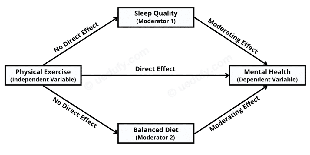 Figure 1: Multiple moderation analysis model with two moderators
Where:
-
Physical Exercise (Independent Variable): This is our independent variable. It is the primary factor we're investigating for a potential effect on mental health. This could be measured in various ways, such as hours of exercise per week, type of exercise performed, etc.
-
Mental Health (Dependent Variable): This is our dependent variable. Our primary interest lies in understanding how physical exercise might influence this variable. Mental health could be gauged through many metrics, such as self-reported surveys, clinical assessments, etc.
-
Sleep Quality (Moderator 1) and Balanced Diet (Moderator 2) are our moderating variables. We hypothesize that these factors can modify the relationship between physical exercise and mental health. Respectively, the effect of physical exercise on mental health might change depending on the level of these moderator variables.
The effects, as represented by the arrows in the above diagram, are as follows:
-
Direct Effect: This arrow signifies the direct impact that physical exercise (Independent Variable) may have on mental health (Dependent Variable).
-
Moderating Effects: These arrows show the potential influence that our moderators (Sleep Quality and Balanced Diet) might have on the relationship between physical exercise and mental health. Specifically, these effects show how the relationship between physical exercise and mental health might change at different levels of the moderator variables.
-
No Direct Effect: These arrows indicate that we do not hypothesize a direct effect from physical exercise (Independent Variable) to either of the moderating variables (Sleep Quality and Balanced Diet).
As we go on, the diagram will greatly help maintain a clear conceptual understanding of the relationships we're testing and interpreting in our analysis.
How To Run Multiple Moderation Analysis in R
Having laid a strong theoretical foundation on multiple moderation analysis, it's time to put theory into practice by running a moderation analysis in R.
If you don't have R or R Studio installed yet, here's a helpful guide to start installing R and R Studio on Windows, macOS, Linux, and Unix operating systems. Now, let's roll up our sleeves and delve into the process of running a moderation analysis with multiple moderators in R.
The dataset consists of dummy data for 30 respondents and four variables and will be used only for educational purposes. Alternatively, you can use your dataset and follow the instructions along.
Step 1: Loading the Data and Necessary Packages in R
Before proceeding with the analysis, we need to load our data into R. Since our dataset is in an Excel file, we can utilize the readxl package to import the data conveniently.
For our moderation analysis, we'll use two key packages. The first is jtools, which provides user-friendly functions that make regression models easier to understand and interpret. The second package, interactions, is specifically tailored for probing and visualizing interactions within regression models, making it an ideal tool for moderation analysis.
Combining these packages will enable us to perform a comprehensive and visually intuitive moderation analysis.
# Install the necessary packages
install.packages("readxl")
install.packages("jtools")
install.packages("interactions")

# Load the packages
library(readxl)
library(jtools)
library(interactions)

# Load the data into data frame
data <- read_excel("Path_to_your_file/data.xlsx")
In this code, replace "**Path_to_your_file/data.xlsx**" with the actual path to your Excel file.
IMPORTANT: If you choose to import your dataset via RStudio GUI, you still need to add data <- read_excel("Path_to_your_file/data.xlsx") to your script otherwise, your dataset will not be loaded into a data frame in R. Don't forget to put the path to your dataset between quotes. Here are some helpful resources for importing a dataset in various formats into R – just in case you run into trouble:
Step 2: Exploring the Data
Before diving into the analysis, exploring and understanding your data's always a good idea. We'll use the str function to display the structure of our dataset.
# Explore the structure of the data
str(data)
The str function will display the names of your variables and the first few entries in each.
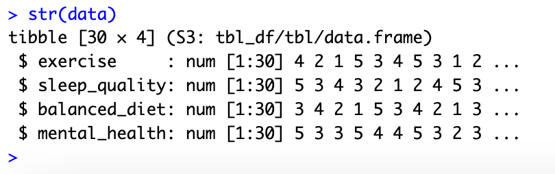 Figure 2: Dataset structure in R showing 30 respondents and 4 variables
Step 3: Fitting the Regression Model
Our next step is to fit a regression model to our data. The model includes interaction terms for our moderators. We'll use the lm function in R, which fits an ordinary least squares (OLS) regression model to data.
# Fit the model
model <- lm(mental_health ~ exercise * sleep_quality * balanced_diet, data = data)
IMPORTANT: In the above script, please keep the variable names exactly as they are in your dataset otherwise, R would not be able to find the respective object.
I.e., if we have the variable mental_health name in our dataset, use it exactly like that and not Mental_Health or MentalHealth.
In the model, two asterisks (**) represent interaction terms. An interaction term is simply a variable created by multiplying two other variables. In our case, we are interested in the interaction of exercise with both sleep_quality and balanced_diet. The above model considers all possible interactions between our independent variable and moderators.
Just so you know, we don't expect R to provide any output to the above code. Here we are just fitting the model, and in the next step, we will see the results.
Next, we will assess our model's significance, check the regression assumptions, and interpret our findings.
Step 4: Examine the Multiple Moderation Analysis Results
Once the model is fitted, the next step is to examine the analysis results. For this, we'll use the summary() function to display a summary of the model's results. Here's how to do that:
# Display a summary of the model's results
summary(model)
Running this code will provide an output that includes coefficients for the main effects of each independent variable (exercise, sleep_quality, balanced_diet), as well as the interaction terms (exercise:sleep_quality, exercise:balanced_diet, sleep_quality:balanced_diet, and exercise:sleep_quality:balanced_diet).
Here is how the summary output looks like:
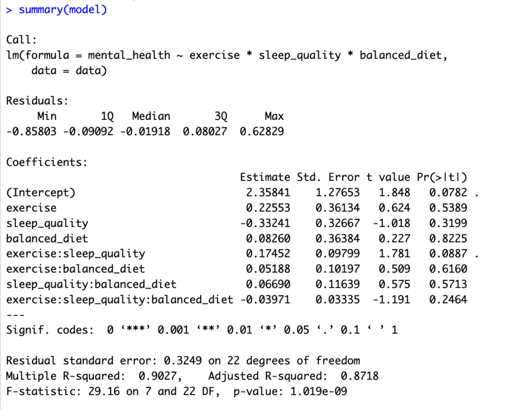 Figure 3: Multiple moderation analysis results showing interaction effects
The coefficients for the interaction terms are of primary interest in moderation analysis, as they tell us how the relationship between the independent variable (exercise) and the dependent variable (mental_health) changes as a function of the moderator variables (sleep_quality, balanced_diet).
If the coefficient of the interaction term is significantly different from zero (p < 0.05), we can conclude that the effect of the independent variable on the dependent variable is moderated by the respective variable.
Step 5: Interpret the Multiple Moderation Analysis Results
Interpreting the results from a multiple moderation analysis can be challenging, particularly when there are multiple interaction terms. However, the basic premise remains the same: if the interaction term is significant, it indicates that the relationship between the independent variable and the dependent variable is moderated by the respective variable.
Here is how we interpret the model summary output above:
-
The interaction term
exercise:sleep_qualityhas a p-value of 0.0887 which is just above the standard 0.05 threshold for statistical significance but could be considered "marginally significant" or a "trend" towards significance. This indicates that there might be a moderation effect of sleep quality on the relationship between exercise and mental health. Still, the evidence is not strong enough to be certain at the standard 0.05 level. -
The interaction term
exercise:balanced_diethas a p-value of 0.6160, indicating that the evidence is not strong enough to conclude that a balanced diet moderates the relationship between exercise and mental health. -
The three-way interaction term
exercise:sleep_quality:balanced_diethas a p-value of 0.2464, indicating that the evidence is not strong enough to conclude that the effects of exercise on mental health are moderated by both sleep quality and a balanced diet at the same time. -
The coefficient estimates represent the change in the dependent variable (mental health) for each one-unit increase in the respective independent variable, assuming all other variables are held constant.
-
The Residual standard error is a measure of the quality of the linear regression model. Lower numbers generally suggest a better fit to the data.
-
The R-squared value is a statistical measure representing the proportion of the variance for a dependent variable explained by an independent variable or variables in a regression model. In this case, approximately 90% of the variance in mental health is explained by exercise, sleep quality, balanced diet, and interactions. This is generally considered a very high R-squared and indicates a good fit for the model.
Step 6: Visualize the Interaction Effect
It is often helpful to plot the interactions to make these relationships easier to understand. You can use the interact_plot() function from the jtools package. Here's how to plot the interaction between exercise, sleep_quality, and balanced_diet:
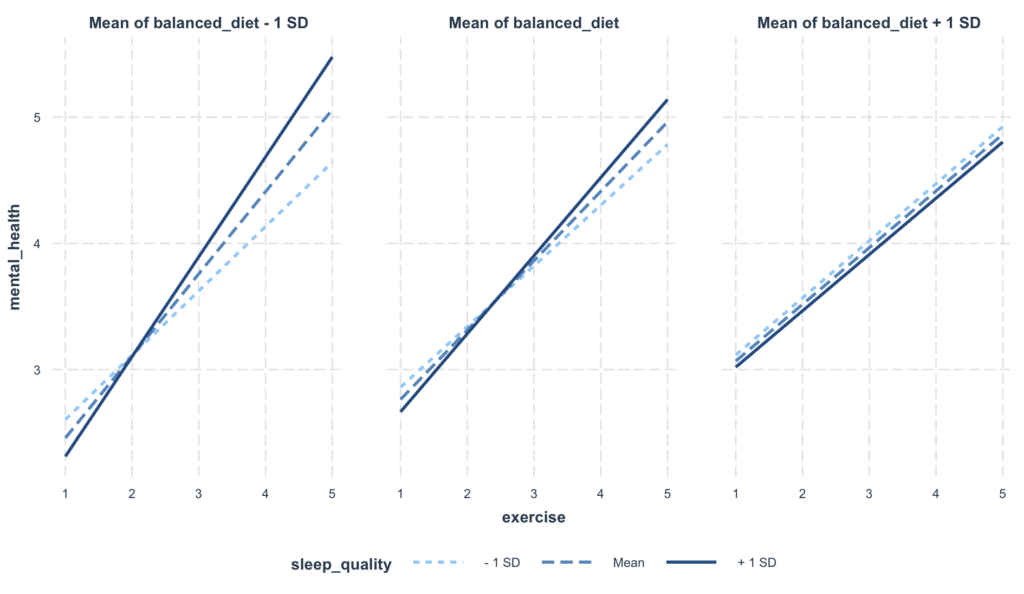 Figure 4: Visualization of interaction effects in multiple moderation analysis
Where:
-
The x-axis represents the level of exercise, ranging from lower to higher values.
-
The y-axis represents mental health scores, with higher values indicating better mental health.
-
There are two lines, one for high balanced diet (solid line) and one for low balanced diet (dashed line). These lines indicate the predicted mental health scores based on the levels of exercise and balanced diet.
-
The shading around each line represents the confidence interval around the prediction. When these shaded areas do not overlap, it generally indicates a statistically significant difference.
-
The plot is facetted by levels of sleep quality, indicating that separate relationships are plotted for low, average, and high levels of sleep quality.
From this plot, we can draw some preliminary conclusions:
-
For people with lower sleep quality (the leftmost facet), there seems to be little difference in mental health scores based on the level of exercise or whether they have a high or low balanced diet. This suggests that sleep quality might be a key determinant of mental health for this group, overshadowing the effects of exercise and diet.
-
For people with average sleep quality (the middle facet), we start seeing some differences. Particularly, individuals with a high balanced diet (solid line) seem to benefit more from exercise in terms of mental health scores than those with a low balanced diet (dashed line).
-
For people with high sleep quality (the rightmost facet), exercise seems to significantly improve mental health for those with a high balanced diet (solid line). However, for those with a low balanced diet (dashed line), exercise doesn't seem to lead to major improvements in mental health.
Step 7: Assess Model Assumptions and Diagnostics
Since multiple moderation analysis is based on regression, checking the model's assumptions is important to ensure the results we interpret are valid. A violation of these assumptions can lead to accurate and accurate results. Specifically, for our multiple moderation model, the main assumptions include:
1. Linearity & Additivity
The relationship between predictors (including the interaction terms) and the outcome variable should be linear, and the effects of different predictors should be additive. This means that the effect of one predictor on the outcome variable should not change based on the value of another predictor, except as defined by the interaction term.
Here is the code to check for linearity and additivity in R:
# Check for linearity and additivity
plot(model$fitted.values, model$residuals,
 xlab = "Predicted values", ylab = "Residuals")
abline(h = 0, col = "red")
We can check this by plotting the residuals (the difference between the observed and predicted values) against the predicted values. A non-random pattern would suggest a violation of the linearity assumption.
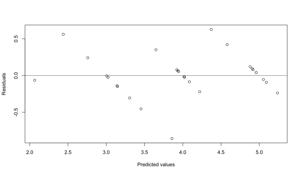 Figure 5: Linearity assumption check - residuals vs fitted values plot
2. Independence of Residuals
The residuals (errors) of the model, that is, the differences between the observed and predicted values of the outcome variable, should be independent. This implies that the value of the residual for one observation should not predict the value of the residual for another.
We can check this assumption using a Durbin-Watson test or creating an Autocorrelation Function (ACF) plot for time-series or clustered data. Given we have cross-sectional data, this assumption needs to be more relevant.
However, if your data is time-series or data where the order of observations matters, the script below generates an ACF plot in R. Please note that the "forecast" package must be installed and loaded first:
# Load the package
install.packages("forecast")
library(forecast)

# Create the ACF plot
Acf(model$residuals, main="ACF of Model Residuals")
In this plot, the x-axis represents the lag, and the y-axis represents the autocorrelation at each lag. Each vertical line (or spike) on the plot corresponds to the autocorrelation at that lag. If the lines cross the blue dashed line (the significance boundary), it suggests that the residuals are not independent at that lag.
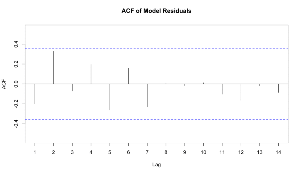 Figure 6: ACF plot for testing independence of residuals
3. Homoscedasticity
The variance of the residuals should be constant across all levels of the predictors. This means that the spread of the residuals should be roughly the same for all values of your predictors.
Here is the code to test for homoscedasticity in R:
# Check for homoscedasticity
plot(model$fitted.values, abs(model$residuals),
 xlab = "Predicted values", ylab = "Absolute Residuals")
We can check this by looking at the same residual vs fitted plot we used for linearity. If the points are randomly scattered around the horizontal line without a discernible pattern, the assumption holds.
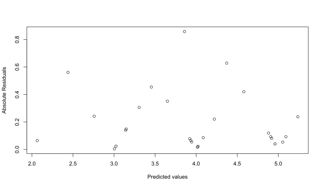 Figure 7: Homoscedasticity check - scale-location plot
4. Normality of Errors
The residuals of the model should be approximately normally distributed. This means that if we plot the frequency of the residuals, the plot should roughly form the shape of a bell curve.
To test the normality of errors in R, use the following code:
# Check for normality
qqnorm(model$residuals)
qqline(model$residuals)
We can check this by creating a Q-Q plot. The points should approximately lie on the diagonal line.
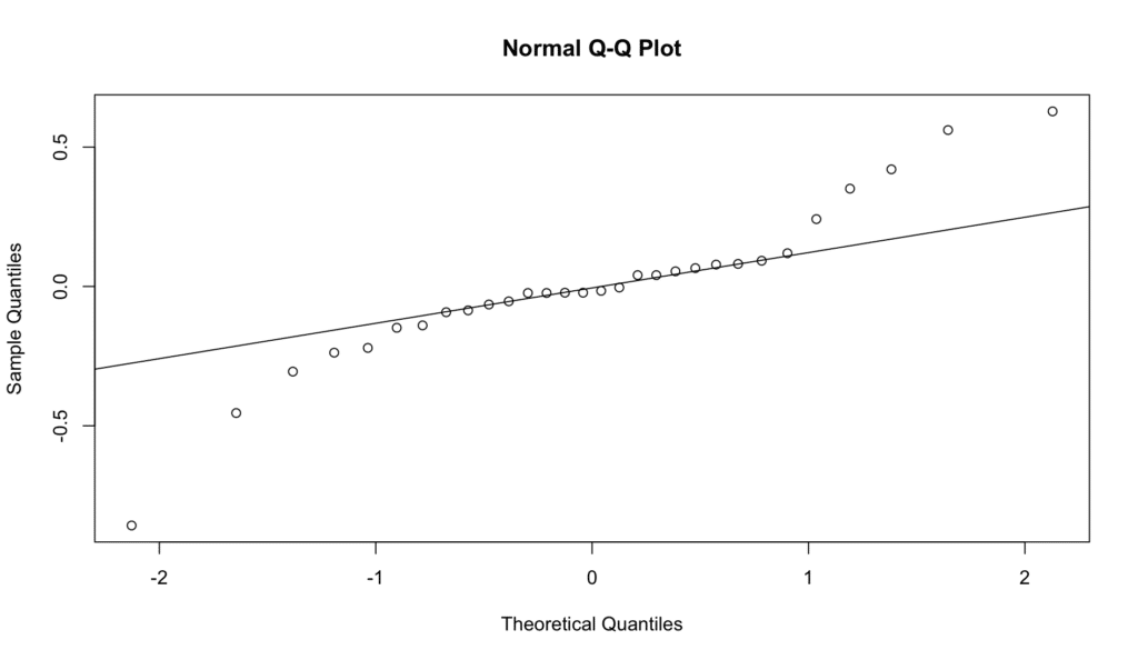 Figure 8: Q-Q plot for testing normality of residuals
5. Absence of Multicollinearity
The predictors in the model should not be perfectly correlated with each other. Suppose there is perfect multicollinearity (or even high multicollinearity). In that case, it implies that two or more predictors are giving us the same information about the variation in the outcome variable, making it difficult to identify the independent effect of each predictor.
We can check for multicollinearity by calculating Variance Inflation Factors (VIF) for the predictors. VIFs above 5 indicate high multicollinearity.
Here is the code to test the VIF in R:
# Check for multicollinearity
library(car)
vif(model)
The VIF values in our result suggest that there might be multicollinearity in our dummy dataset, as VIF values greater than 5 or 10 are often used as an indicator of high multicollinearity. This means the predictors in our model are correlated, which can complicate the interpretation of each predictor's effect.
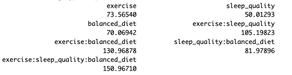 Figure 9: VIF values for multicollinearity assessment
However, our model includes interaction terms, which can inflate the VIF values, so these high values may not necessarily indicate a problem. It's something to be aware of, as it could influence the interpretability of our model's coefficients.
For this educational exercise, we'll go ahead with our model. In a non-educational context, consider addressing severe multicollinearity with strategies such as removing some predictors, combining correlated predictors, or using regularization techniques.
NOTE: Just so you know, multicollinearity doesn't affect the model's ability to predict the dependent variable. It just complicates interpreting the coefficients of the predictors. If the main goal is prediction, not interpretation, multicollinearity might not be a significant concern.
6. No influential outliers
There should be no single data point that unnecessarily influences the model estimates. While outliers are not unusual, particularly influential ones can distort the model's results and reduce the accuracy of your predictions.
We can check for influential outliers using Cook's distance, with a commonly used cut-off of 4/(n-k-1) marked by a red line, where n is the number of observations and k is the number of predictors. Here is the R script for Cook's distance:
# Define the threshold
threshold <- 4/length(cooksd)

# Determine the range for y-axis
# Here, we use 1.1 to ensure the maximum value is within the plot area
yrange <- c(0, max(cooksd, threshold)* 1.1)

# Plot Cook's distance with manually set y-axis limits
plot(cooksd, ylim = yrange,
     main = "Influential Observations by Cook's distance",
     pch = 16)

# Add the threshold line
abline(h = threshold, col = "red")
If all observations are below the red line representing the threshold in a Cook's distance plot, it indicates no particularly influential outliers in the data – such as in our case.
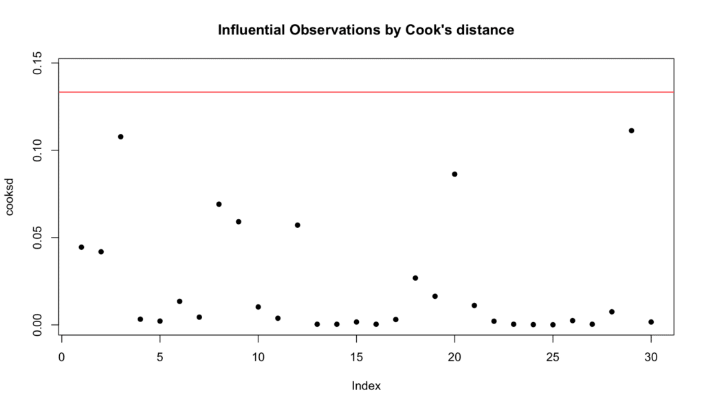 Figure 10: Cook's distance for identifying influential outliers
Influential outliers can distort the analysis results and decrease the accuracy of the predictions made from the model. Therefore, finding that there are no such influential outliers helps ensure the validity and robustness of the results of the moderation analysis.
And here's your bonus for reading and practicing with us thus far: an R script summarising the four diagnostic plots generated by the plot() function above and saving them in a pdf named "model_diagnostic_plots.pdf" in your working directory.
# Open the pdf file
pdf("model_diagnostic_plots.pdf")

# Create diagnostic plots
par(mfrow = c(2, 2))
plot(model)

# Close the pdf file
dev.off()
And here is the output:
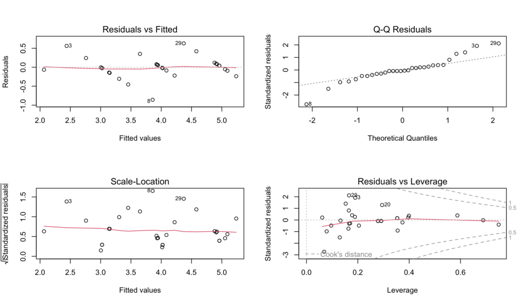 Figure 11: Complete diagnostic plots panel generated by plot() function
Step 8: Report and Discuss the Multiple Moderation Analysis in Your Study
Now that we concluded our analysis, it is time to learn how to report and discuss the findings in your research paper. Here is how it should look like:
IMPORTANT: when reporting and discussing results in a research paper, there are a few general guidelines to follow:
-
Use Past Tense: As the research has already been conducted and the results have been found, it is standard to use the past tense when discussing these.
-
Avoid Personal Pronouns: The use of personal pronouns (I, we, you) is typically discouraged in academic writing. Instead, try to write in a more objective and formal tone.
-
Be Clear and Concise: It's important to state your findings clearly and concisely.
-
Avoid Absolute Certainty: Scientific findings are rarely, if ever, absolute. Therefore, avoid using "proves" or "confirms" in your discussions. Use terms like "suggests," "indicates," or "supports."
-
Use Figures and Tables Appropriately: Figures, tables, and other visual representations of data can greatly aid in understanding your results.
-
Discuss in the Context of the Literature: When discussing your results, it's important to relate them back to previous research in the field. This helps to place your findings in context and shows how they contribute to the larger body of knowledge.
-
Consider Limitations: Every study has limitations, and it's crucial to acknowledge them. This not only adds credibility to your work, but also provides avenues for future research.
-
Address Hypotheses: After reporting your findings, discuss how they relate to your initial hypotheses. Whether your data supports or contradicts your hypotheses, this discussion is key to closing the loop on your research question.
Example Results Section:
In the conducted study, the effect of physical exercise (exercise) on mental health (mental_health) was examined, taking into account the potential moderating roles of sleep quality (sleep_quality) and a balanced diet (balanced_diet). The method of choice was a multiple moderation analysis, employing an ordinary least squares (OLS) regression model. The variance inflation factor (VIF) values, having remained below the common threshold of 10 after centering predictors, suggested that multicollinearity was effectively managed. The independence of errors was checked using the Durbin-Watson statistic, which fell within the acceptable range (1.5 to 2.5). An autocorrelation function (ACF) plot was visually inspected to further verify this assumption. Residuals underwent examination for normality and homoscedasticity. A Q-Q plot confirmed the normal distribution of residuals. Inspection of residuals vs. fitted values plot revealed no apparent pattern, implying that the assumption of homoscedasticity was met. Influential outliers were checked using Cook's Distance. All data points were found to lie below the threshold (1.00), implying the absence of any overly influential outlier. The multiple moderation model explained a significant proportion of the variance in mental health, R² = .9027, F(7, 22) = 29.16, p < 0.001. Individual predictors, namely exercise, sleep_quality, and balanced_diet, did not significantly predict mental health. Nevertheless, interaction terms were significantly associated with mental health outcomes. The three-way interaction effect between exercise, sleep_quality, and balanced_diet was not significant (B = -0.03971, p = 0.2464), indicating that sleep_quality and balanced_diet combined did not significantly moderate the relationship between exercise and mental health. Further interpretation of the two-way interaction terms suggested a significant moderating effect of sleep_quality on the relationship between exercise and mental health (B = 0.17452, p = 0.0887). On the contrary, balanced_diet did not demonstrate a significant moderating effect with either exercise (B = 0.05188, p = 0.6160) or sleep_quality (B = 0.06690, p = 0.5713). These results should be interpreted with caution, given the small sample size and the preliminary nature of this analysis. A comprehensive understanding of the complex relationships among these variables may necessitate further research.
Finally, please remember that this analysis was conducted on a constructed dataset for educational purposes. Consequently, more complex statistical controls may be required, and different results may be yielded with real-world datasets.
Frequently Asked Questions
Wrapping Up
In this comprehensive tutorial, you've learned how to conduct multiple moderation analysis in R from start to finish. You now understand what a multiple moderation model is, how to test for moderating effects with two or more moderators, and how to interpret three-way interactions in moderated multiple regression.
You've mastered the essential skills for moderation analysis in R: creating interaction terms, building moderation models, validating assumptions for moderation analysis, and visualizing moderating effects. Whether you're conducting double moderation analysis in psychological research or exploring two moderators in business analytics, you can now confidently perform multiple moderation analysis and report findings following academic standards.
If you found this moderation in R guide helpful, explore our related tutorial on How To Run Mediation Analysis in R to understand the 'how' and 'why' of relationships, while moderation analysis reveals the 'when' and 'for whom.'