How to Run Mediation Analysis in R: 7 Easy Steps

Learning how to run mediation analysis in R is essential for understanding indirect effects in your research. This complete guide shows you how to perform mediation analysis in R and mediation in R using the lavaan package and R mediation techniques, with a step-by-step walkthrough using a dummy dataset of 30 respondents.

Whether you need to run mediation analysis R for your thesis, understand R mediation analysis for publication, or build a mediation model in R for exploratory research, this tutorial covers everything. We'll show you how to use the mediation package in R with lavaan, interpret path coefficients (a, b, c), and visualize results with professional diagrams.

In seven easy-to-follow steps, you'll master mediation R workflows using both the lavaan and mediation packages, and learn how to conduct complete R mediation analysis from data import to interpretation.

Lesson Outcomes

By the end of this lesson, you will be able to:

• Understand the concept of mediation analysis and its purpose in exploring indirect effects.

• Visualize a mediation model using a simple diagram.

• Install and load necessary R packages for mediation analysis

• Import and explore a dataset in R, computing descriptive statistics and correlations among variables.

• Specify a mediation model in R.

• Estimate and fit the mediation model to your dataset in R

• Interpret the results of a mediation analysis, including direct effects, indirect effects, and total effects.

• Create a visualization of the mediation analysis results in R.

• Apply the mediation analysis process to your own research questions and datasets.

Are you ready? Let's get started and explore the process!

What is Mediation Analysis?

Before we start crunching numbers, let's briefly discuss what mediation analysis is. It's a statistical technique that helps us understand how an independent variable (X) influences a dependent variable (Y) through a mediator variable (M).

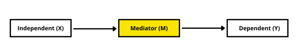
Basic mediation model diagram with X→M→Y paths.

Mediation analysis is particularly useful for determining if the effect of X on Y is entirely, partially, or not mediated by M.

Our Dataset: A Brief Overview

In our example, we'll be working with a dataset of 30 respondents. Let's say these respondents are employees, and we want to study the relationship between job satisfaction (X), job performance (Y), and workplace motivation (M).

We hypothesize that job satisfaction influences job performance indirectly through workplace motivation. So, we're going to perform a mediation analysis to see if this is true.

To visualize our hypothesis, we can create a simple diagram with three variables: job satisfaction (X), workplace motivation (M), and job performance (Y).

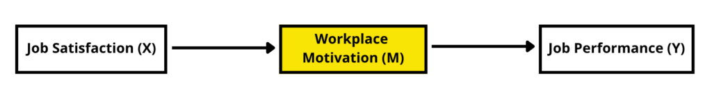
Mediation model example: job satisfaction → workplace motivation → job performance.

In this diagram, the arrow from X to M represents the effect of job satisfaction on workplace motivation (a path). The arrow from M to Y represents the effect of workplace motivation on job performance (b path). The indirect effect of job satisfaction on job performance through workplace motivation is the product of the a and b paths (a *b).

How To Run Mediation Analysis in R

Now that we have a clear understanding of our dataset and hypothesis, let's jump into R and start working with the data.

Step 1: Install and Load Packages

First, we'll need to install and load the necessary packages for conducting mediation analysis in R as well as visualizing the results:

# Install packages
install.packages("psych")
install.packages("lavaan")
install.packages("ggplot2")
install.packages("readxl")
install.packages("semPlot")

# Load packages
library(psych)
library(lavaan)
library(ggplot2)
library(readxl)
library(semPlot)

Here is a brief description of the above packages:

-**psych:**Package for performing psychological and psychometric analyses, such as factor analysis and descriptive statistics.

-**lavaan:**Package for structural equation modeling (SEM) with user-friendly syntax and a range of fit indices.

-**ggplot2:**Flexible data visualization package based on the Grammar of Graphics for creating complex and customizable plots.

-**readxl:**Lightweight package for importing Excel files (.xls and .xlsx) into R data frames.

-**semPlot:**Visualization tool for creating path diagrams of structural equation models (SEMs) with customization options.

Step 2: Import and Explore the Dataset

Next, we'll import our dataset into R and look at the first few rows to familiarize ourselves with the data. You may use your own dataset, or download the practice dataset from the sidebar (for educational purposes only).

NOTE: If your dataset is an Excel .xlsx file, use the following syntax:

# Import the dataset
data <- read_excel("path/to/your/dataset.xlsx")

#Explore dataset
head(data)

• If your dataset is an Excel .csv file, use the following syntax:

# Import dataset
data <- read.csv("path/to/your/dataset.csv")

# Explore dataset
head(data)

Assuming our dataset contains three columns – job_satisfaction, workplace_motivation, and job_performance – the output should look something like this:

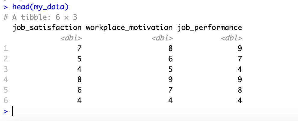
Dataset preview showing the first 6 rows of the mediation analysis dataset in R.

Step 3: Descriptive Statistics and Correlations

Before we run the mediation analysis, let's compute some descriptive statistics and correlations for our variables.

# Descriptive statistics
summary(data)

# Correlations
correlations <- cor(data)
print(correlations)

This will give us an overview of our variables' mean, standard deviation, and correlations.

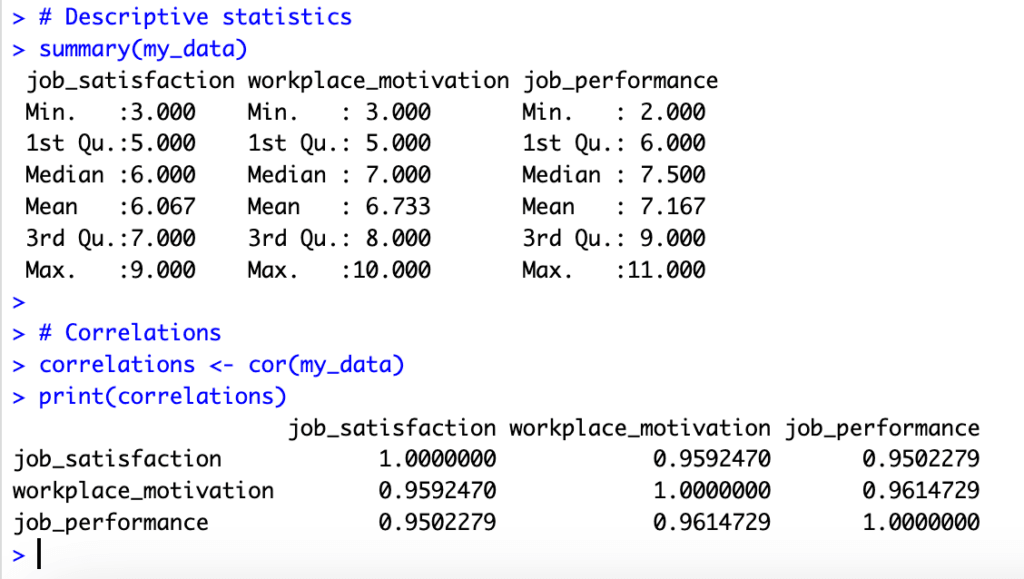
Descriptive statistics and correlation matrix output in R for mediation variables.

Performing descriptive statistics and correlation analysis prior to mediation analysis is important for several reasons:

-Data understanding: Descriptive statistics provide a summary of your dataset and help you understand the central tendency, dispersion, and shape of the distribution for each variable. This understanding is crucial before diving into more complex analyses like mediation analysis, as it helps you identify any potential issues or outliers in the data.

-Assumptions checking: Many statistical techniques, including mediation analysis, rely on certain assumptions about the data. Descriptive statistics can help you assess whether these assumptions are met. For example, normality of the variables is often an assumption in mediation analysis, and you can examine this through descriptive statistics like skewness and kurtosis.

-Preliminary insights: Correlation analysis provides an initial understanding of the relationships between your variables. It helps you examine the strength and direction of the associations, which can be useful in generating hypotheses or informing the mediation model. Strong correlations between the independent variable (X) and the mediator (M), as well as between the mediator (M) and the dependent variable (Y), might indicate the presence of mediation effects.

-Multicollinearity assessment: Examining correlations can also help you detect multicollinearity, a situation where two or more predictor variables are highly correlated. Multicollinearity can cause issues in mediation analysis, as it may lead to unstable estimates or inflated standard errors. By identifying multicollinearity early on, you can address it before proceeding with the mediation analysis.

Step 4: Specify the Mediation Model

Now that we better understand our dataset, it's time to specify the mediation model. We'll use the R lavaan package to define the model using the following syntax:

mediation_model <- '
 # Direct effects
 workplace_motivation ~ a*job_satisfaction
 job_performance ~ c * job_satisfaction + b*workplace_motivation

 # Indirect effect (a * b)
 indirect := a*b

 # Total effect (c + indirect)
 total := c + indirect
'

In this model, we define the direct effects of job satisfaction (X) on workplace motivation (M) and job performance (Y). We also specify the indirect effect (a*b) and the total effect (c + indirect).

NOTE: If you wonder why you're not getting any output for the above R script is because this only specifies the mediation model as a string but does not perform the analysis or print any results. The actual mediation analysis in R will be performed in the next step.

Step 5: Estimate the Mediation Model

With our mediation model specified, we can now estimate it using the lavaan package. We'll fit the model to our dataset and then summarize the results.

# Estimate the mediation model
mediation_results <- sem(mediation_model, data = data)

# Summarize the results
summary(mediation_results, standardized = TRUE, fit.measures = TRUE)

The summary will show the estimated direct effects (a, b, and c paths), the indirect effect (a*b), and the total effect (c + indirect) along with their significance levels – as seen below:

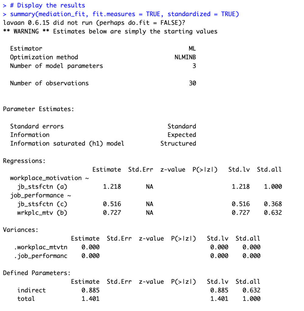
Lavaan SEM output displaying mediation analysis results with path estimates and significance levels.

Alright, but what do all these numbers mean? Let's discuss this next.

Step 6: Interpret Mediation Output in R

Based on the output of your mediation analysis using the dummy dataset we used in this lesson, here's how to interpret mediation analysis results in R:

Parameter Estimates:

• Path a (job satisfaction -> workplace motivation): The estimated coefficient for the direct effect of job satisfaction (X) on workplace motivation (M) is 1.218. This suggests that, on average, a one-unit increase in job satisfaction is associated with a 1.218-unit increase in workplace motivation, assuming a linear relationship. The standardized coefficient (Std.all) is 1.000, which indicates a strong positive relationship between job satisfaction and workplace motivation.

• Path b (workplace motivation -> job performance): The estimated coefficient for the direct effect of workplace motivation (M) on job performance (Y) is 0.727. This suggests that, on average, a one-unit increase in workplace motivation is associated with a 0.727-unit increase in job performance, assuming a linear relationship. The standardized coefficient (Std.all) is 0.632, which indicates a moderate positive relationship between workplace motivation and job performance.

• Path c (job satisfaction -> job performance): The estimated coefficient for the direct effect of job satisfaction (X) on job performance (Y) without considering the mediation effect is 0.516. This suggests that, on average, a one-unit increase in job satisfaction is associated with a 0.516-unit increase in job performance, assuming a linear relationship. The standardized coefficient (Std.all) is 0.368, which indicates a weak to moderate positive relationship between job satisfaction and job performance.

Defined Parameters:

• Indirect effect (a*b): The estimated indirect effect of job satisfaction (X) on job performance (Y) through workplace motivation (M) is 0.885. This suggests that, on average, a one-unit increase in job satisfaction results in a 0.885-unit increase in job performance indirectly through its effect on workplace motivation. The standardized indirect effect (Std.all) is 0.632, which indicates a moderate positive relationship.

• Total effect (c + indirect): The estimated total effect of job satisfaction (X) on job performance (Y), considering both the direct and indirect effects, is 1.401. This suggests that, on average, a one-unit increase in job satisfaction is associated with a 1.401-unit increase in job performance when considering both the direct and indirect effects. The standardized total effect (Std.all) is 1.000, which indicates a strong positive relationship.

Just so you know, the results presented here are based on a fictional dataset created for demonstration purposes only, and the interpretations should not be considered meaningful. However, the process of interpreting the mediation analysis results remains the same for real-life datasets.

Step 7: Visualize Mediation in R

To make our results more accessible, let's create a diagram using the ggplot2 package:

# Load the necessary libraries
library(ggplot2)

# Create a bar plot to visualize the path coefficients
ggplot(path_data, aes(x = path, y = coefficient, fill = path)) +
 geom_bar(stat = "identity", position = position_dodge()) +
 geom_text(aes(label = round(coefficient, 3)), vjust = -0.3, size = 4) +
 theme_minimal() +
 theme(legend.position = "none") +
 ylab("Coefficient") +
 xlab("Path") +
 ggtitle("Mediation Analysis Results")

The above script will create a bar chart displaying the coefficients for each path in our mediation model:

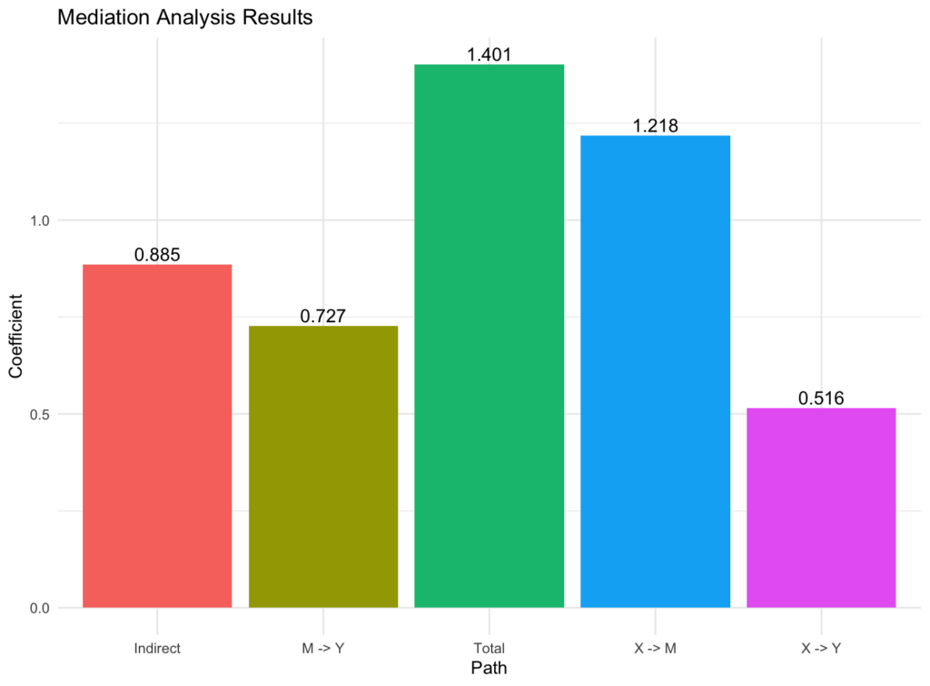
Bar chart showing path coefficients (a, b, c, indirect, total) from mediation analysis.

The bar chart we created above is a good representation of our mediation analysis. Still, we can push this further and generate a mediation diagram with the path estimates displayed on the arrows, making it easier to interpret the relationships between the variables using the following R script:

# Load the necessary libraries
library(ggplot2)
library(semPlot)

# Create a bar plot to visualize the path coefficients
bar_plot <- ggplot(path_data, aes(x = path, y = coefficient, fill = path)) +
 geom_bar(stat = "identity", position = position_dodge()) +
 geom_text(aes(label = round(coefficient, 3)), vjust = -0.3, size = 4) +
 theme_minimal() +
 theme(legend.position = "none") +
 ylab("Coefficient") +
 xlab("Path") +
 ggtitle("Mediation Analysis Results")

# Plot the bar plot
print(bar_plot)

# Plot the mediation diagram with path estimates
semPaths(mediation_fit, whatLabels = "est", style = "lisrel", intercepts = FALSE)

This will generate a mediation diagram with the path estimates displayed on the arrows, making it easier to interpret the relationships between the variables in our model:

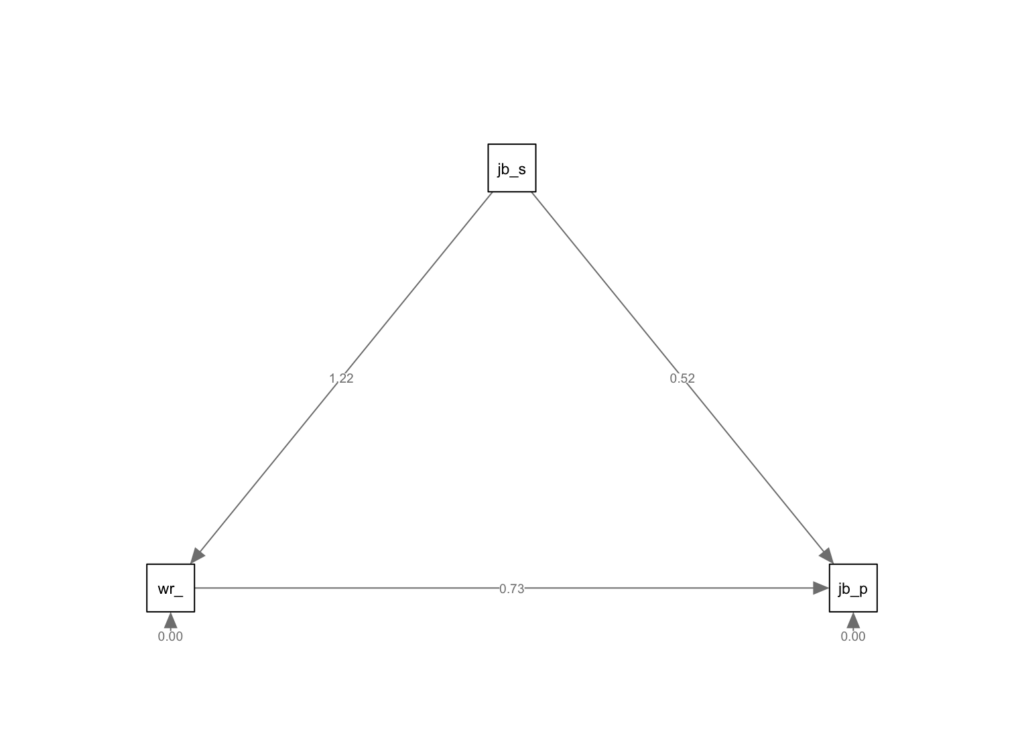
Path diagram created with semPlot showing mediation model with estimated coefficients.

Here's a brief explanation of how to interpret the above diagram:

-**X -> M (a path):**This arrow shows the effect of job satisfaction (X) on workplace motivation (M). A positive number means that as job satisfaction increases, workplace motivation also increases. A negative number indicates that as job satisfaction increases, workplace motivation decreases. The magnitude of the number reflects the strength of this relationship.

-**M -> Y (b path):**This arrow represents the effect of workplace motivation (M) on job performance (Y), assuming job satisfaction (X) is held constant. A positive number means that as workplace motivation increases, job performance also increases. A negative number indicates that as workplace motivation increases, job performance decreases. The magnitude of the number reflects the strength of this relationship.

-**X -> Y (c path):**This arrow shows the direct effect of job satisfaction (X) on job performance (Y), without considering the mediator (workplace motivation). A positive number means that as job satisfaction increases, job performance also increases. A negative number indicates that as job satisfaction increases, job performance decreases. The magnitude of the number reflects the strength of this relationship.

To interpret the results, consider the signs (positive or negative) and the magnitudes of the path coefficients. A larger absolute value indicates a stronger relationship between the variables.

If the indirect effect (a* b) is significant, it suggests that workplace motivation mediates the relationship between job satisfaction and job performance. In this case, part of the effect of job satisfaction on job performance can be explained through workplace motivation.

Frequently Asked Questions

Wrapping Up

In this comprehensive guide, you've learned how to run mediation analysis in R using the lavaan package with a complete 7-step process. From installing packages to visualizing results, you now understand how to perform mediation in R, interpret path coefficients (a, b, c), and test indirect effects.

The mediation analysis R workflow we covered—from data import through R mediation analysis interpretation—provides you with a solid foundation for investigating indirect effects in your research. Whether you're building a mediation model in R for your thesis or exploring mediating mechanisms in real-world data, the lavaan package offers the flexibility and precision you need.

Need help with related analyses? Check out our guides on mediation analysis in SPSS, moderation analysis in R, or learn about mediators vs moderators to deepen your understanding of advanced statistical techniques.

References

Baron, R. M., & Kenny, D. A. (1986). The moderator-mediator variable distinction in social psychological research: Conceptual, strategic, and statistical considerations. Journal of Personality and Social Psychology, 51(6), 1173-1182.
Rosseel, Y. (2012). lavaan: An R package for structural equation modeling. Journal of Statistical Software, 48(2), 1-36.
Preacher, K. J., & Hayes, A. F. (2008). Asymptotic and resampling strategies for assessing and comparing indirect effects in multiple mediator models. Behavior Research Methods, 40(3), 879-891.