Multiple linear regression extends simple regression by allowing you to predict an outcome using two or more predictor variables simultaneously. This is essential for thesis research where real-world phenomena are rarely explained by a single factor. Whether you're predicting academic performance from study habits, sleep, and attendance, or forecasting sales from advertising, pricing, and seasonality, multiple regression reveals which predictors matter most and how they work together.
Unlike simple regression which answers "Does X predict Y?", multiple regression answers the more realistic question: "Do X₁, X₂, and X₃ together predict Y, and which predictor has the strongest effect?" This makes it one of the most widely used statistical techniques in dissertation research across psychology, education, business, health sciences, and social sciences.
This comprehensive guide shows you how to perform multiple linear regression in Excel using the Analysis ToolPak, interpret output correctly (including adjusted R² and individual predictor significance), detect multicollinearity problems, check assumptions, and report findings in APA 7th edition format. You'll also learn the critical limitations of Excel and when you need SPSS or R instead.
Key Takeaways:
- Multiple regression predicts Y from 2+ predictor variables simultaneously
- Always report adjusted R² (not regular R²) because it corrects for number of predictors
- Check multicollinearity first using correlation matrix (predictors should have r < 0.80)
- A significant overall model (F-test) does not mean all individual predictors are significant
- Excel handles standard multiple regression well but cannot do stepwise, hierarchical, or logistic regression
Before you begin: This guide assumes you understand simple linear regression - read that first if you're new to regression. You'll also need Excel with the Analysis ToolPak installed. If you haven't enabled it yet, see our guide on how to add Data Analysis in Excel.
What is Multiple Linear Regression?
Multiple linear regression is a statistical method that models the relationship between two or more independent variables (predictors, X₁, X₂, X₃...) and one dependent variable (outcome, Y) by fitting a linear equation to observed data. It extends simple regression to account for multiple factors that might influence your outcome.
The Multiple Regression Equation
If you've been reading statistics textbooks or watching tutorials, you may have noticed the regression formula written differently depending on the source. Don't worry - both versions are correct! The difference is simply a notation convention, and understanding both will help you read any statistics resource with confidence.
In theoretical statistics books, you'll typically see Greek letters (beta symbols). This notation represents the true population parameters - the "real" values that exist in the entire population we're trying to estimate:
In applied guides and Excel tutorials (including this one), you'll often see Roman letters (a and b). This notation represents the sample estimates - the actual values Excel calculates from your data as estimates of those population parameters:
The bottom line: When you see β₀ in a textbook and "Intercept" in Excel, they're referring to the same thing. When your professor writes β₁ on the board and Excel shows a coefficient of 2.15, that's the same concept. Excel labels its output simply as "Coefficients" regardless of which notation your textbook uses.
Where:
- Y = Dependent variable (what you're predicting)
- X₁, X₂, X₃ = Independent variables (your predictors)
- β₀ or a = Intercept (expected Y value when all X variables = 0)
- β₁, β₂, β₃ or b₁, b₂, b₃ = Slope coefficients (change in Y for each 1-unit increase in that X, holding other predictors constant)
- ε = Error term (unexplained variation)
For example, if you're predicting exam scores from study hours, sleep, and class attendance:
This means: Each additional study hour increases exam score by 1.75 points (holding sleep and attendance constant), each additional hour of sleep adds 0.52 points, and each additional class attended adds 2.36 points.
The Key Advantage: "Holding Other Variables Constant"
The phrase "holding other variables constant" (also called "controlling for") is what makes multiple regression powerful. In simple regression, if study hours predicts exam scores, you can't tell if it's truly study hours or something correlated with it (like attendance). Multiple regression separates these effects:
- Simple regression: "Students who study more score higher" (but maybe they also attend more classes)
- Multiple regression: "Students who study more score higher, even when we account for their attendance"
This allows you to isolate the unique contribution of each predictor - essential for making causal arguments in your thesis Discussion chapter.
When to Use Multiple Linear Regression for Your Thesis
Use multiple linear regression when your research meets these criteria:
1. Research Question Requirements:
- You want to predict Y using multiple factors simultaneously
- You want to control for confounding variables
- You want to determine which predictors matter most
- You want to compare the relative importance of different predictors
2. Variable Requirements:
- Two or more continuous predictors (X₁, X₂, etc.): Interval or ratio scale
- One continuous outcome (Y): Interval or ratio scale
- Minimum sample size: n ≥ 50 + 8k (where k = number of predictors)
3. Research Examples by Discipline:
- Psychology: Do therapy hours, medication adherence, AND social support predict depression reduction?
- Education: Do study hours, sleep quality, AND class attendance predict exam scores?
- Business: Do advertising budget, price, AND competitor activity predict sales revenue?
- Health Sciences: Do exercise, diet quality, AND medication compliance predict weight loss?
- Social Sciences: Do income, education, AND social networks predict life satisfaction?
Simple vs Multiple Linear Regression: Which Do You Need?
Before proceeding, make sure multiple regression is the right choice for your research question:

Figure 1: Decision flowchart for selecting simple linear regression (one predictor) or multiple linear regression (two or more predictors) based on your research question
| Feature | Simple Linear Regression | Multiple Linear Regression |
|---|---|---|
| Number of predictors | 1 independent variable | 2 or more independent variables |
| Equation | Y = a + bX | Y = a + b₁X₁ + b₂X₂ + b₃X₃... |
| Research question | "Does study time predict exam scores?" | "Do study time, sleep, AND attendance together predict exam scores?" |
| Controls for confounders | No | Yes - isolates unique effects |
| Compares predictor importance | N/A (only one predictor) | Yes - which predictor matters most? |
| Key statistic | R² | Adjusted R² (corrects for number of predictors) |
| Additional assumption | None | No multicollinearity between predictors |
| Excel capability | Full support | Full support (but no VIF calculation) |
Table 1: Simple vs. Multiple Linear Regression Comparison
Use Simple Linear Regression when:
- You have only one predictor variable
- Your research question focuses on one specific relationship
- You're doing preliminary analysis before adding more predictors
- Example: "Does advertising budget predict sales?"
Use Multiple Linear Regression when:
- You have two or more predictor variables
- You want to control for confounding variables
- You need to compare the relative importance of predictors
- You're testing a theoretical model with multiple factors
- Example: "Do advertising budget, price, AND seasonality together predict sales, and which matters most?"
Different research question? If you're comparing group means rather than predicting a continuous outcome, see our guide on choosing between T-Test and ANOVA.
Sample Dataset for This Tutorial
Throughout this guide, we'll use a realistic thesis dataset examining how multiple factors predict exam performance for 30 university students. This demonstrates a typical research question: "Do study hours, sleep quality, and class attendance together predict academic performance?"
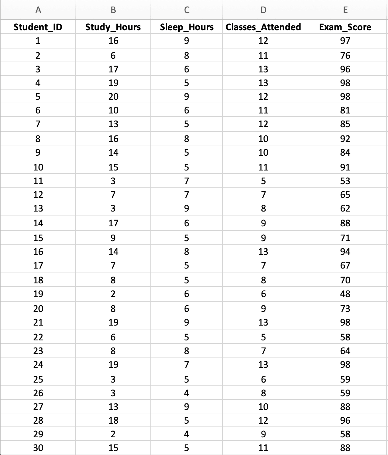
Figure 2: Sample dataset with 30 students showing three predictor variables (Study Hours, Sleep Hours, Classes Attended) and one outcome variable (Exam Score)
Dataset characteristics:
- Sample size: n = 30 students (minimum for 3 predictors, but adequate for teaching)
- Independent variables (X):
- X₁: Study Hours per week (range: 2-20 hours)
- X₂: Sleep Hours per night (range: 4-9 hours)
- X₃: Classes Attended out of 15 (range: 5-15 classes)
- Dependent variable (Y): Exam Score (range: 45-98 points)
- Research question: Do study hours, sleep, and attendance together predict exam performance, and which predictor matters most?
Create your own dataset:
- Enter your data in columns (all X variables + Y variable)
- Include headers in row 1
- Minimum n = 50 + 8k observations recommended (k = number of predictors)
- Ensure all variables are continuous (no categorical variables in standard multiple regression)
- Check for missing values before analysis. If you have incomplete cases, see how to handle missing data in Excel before running regression.
Note on Sample Size: This teaching dataset uses n = 30 for demonstration purposes. For actual thesis research with 3 predictors, you should have at least n = 74 (using the formula n ≥ 50 + 8k). The example shows strong relationships for clarity - real behavioral science data typically shows weaker effects.
How to Calculate Multiple Linear Regression in Excel (Step-by-Step)
The Analysis ToolPak provides comprehensive multiple regression output including R², adjusted R², F-statistic, individual predictor significance, and residuals. This is the recommended method for thesis research.
Analysis Workflow Overview
Before running multiple regression, follow this sequence:
- Check multicollinearity between predictors (correlation matrix, r < 0.80)
- Run the regression using Analysis ToolPak
- Evaluate overall model (F-test significance, adjusted R²)
- Evaluate individual predictors (p-values for each coefficient)
- Check assumptions (residual plots for normality, homoscedasticity)
- Report in APA format (model fit, then individual predictors)
This sequence ensures you identify multicollinearity problems before investing time interpreting coefficients that may be unstable or misleading.
Note on Regional Settings: Excel formulas use different argument separators depending on your locale. US/UK Excel uses commas:
=STDEV.S(A1:A30)while European Excel uses semicolons:=STDEV.S(A1:A30). If a formula returns an error, try swapping commas for semicolons (or vice versa). To check or change your settings:
- Windows: File → Options → Advanced → "Use system separators"
- Mac: System Preferences → Language & Region → Advanced → Number separators
Step 1: Verify Analysis ToolPak is Enabled
If you haven't used the Analysis ToolPak before, enable it first:
- Click File → Options
- Select Add-ins (left sidebar)
- At the bottom, select Excel Add-ins from "Manage" dropdown
- Click Go
- Check Analysis ToolPak and click OK
Need detailed instructions? See our complete guide: How to Enable Data Analysis in Excel
Step 2: Access Data Analysis and Select Regression
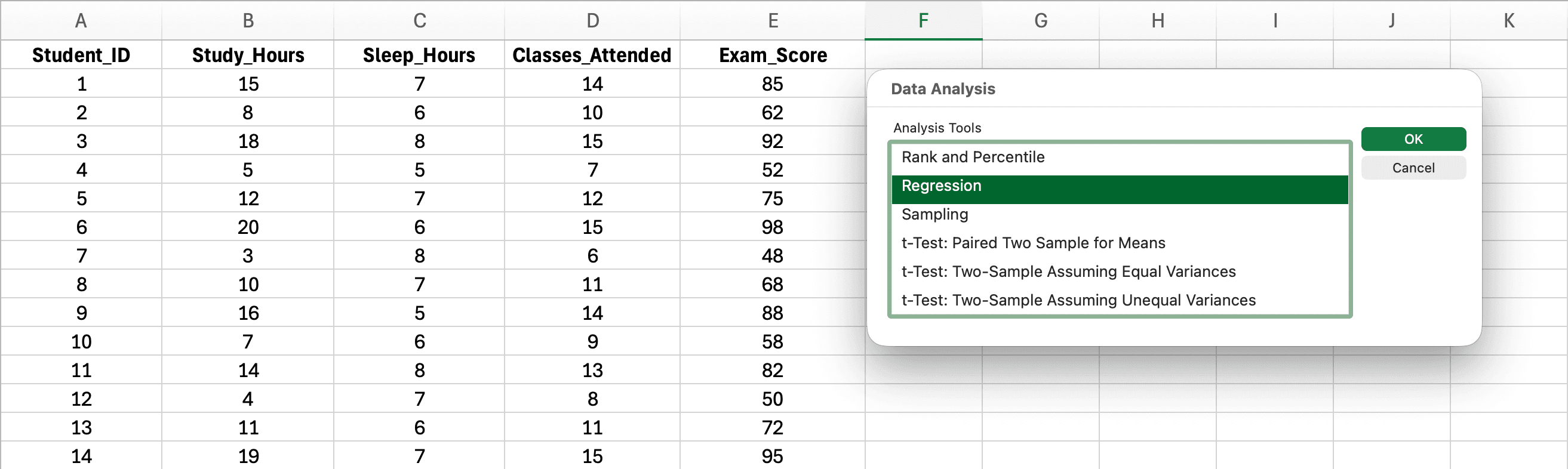
Figure 3: Accessing Data Analysis from the Data tab and selecting Regression
- Click the Data tab in Excel ribbon
- Click Data Analysis (far right side)
- Scroll down and select Regression
- Click OK
Step 3: Configure the Regression Dialog for Multiple Predictors
This is where multiple regression differs from simple regression - you'll select multiple columns for Input X Range.
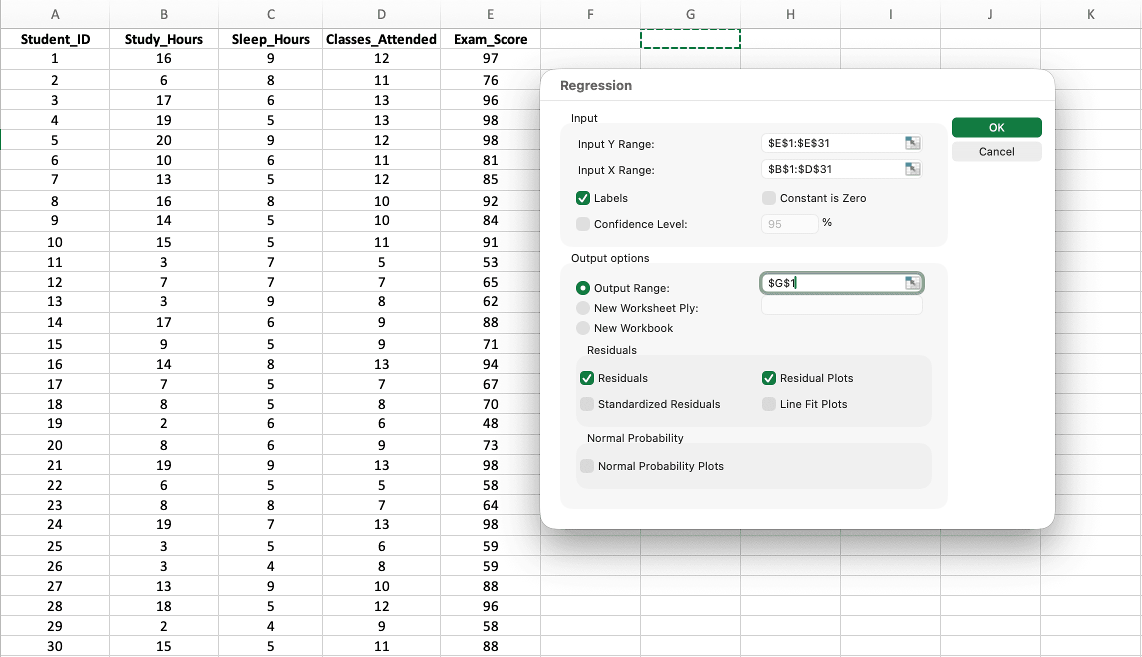
Figure 4: Regression dialog configured for multiple predictors - note the Input X Range spans three columns (B1:D31)
Critical settings:
-
Input Y Range: Select your dependent variable column including header (e.g.,
E1:E31for Exam_Score) -
Input X Range: Select ALL predictor columns together including headers (e.g.,
B1:D31for Study_Hours, Sleep_Hours, AND Classes_Attended)- Important: Select all X columns as one continuous range, not separately
- The columns must be adjacent (side by side)
-
Labels: Check this box (tells Excel row 1 contains variable names)
-
Output Range: Click a cell where results should appear (e.g.,
G1) -
Residuals: Check this for assumption checking
-
Click OK
Note on Regional Settings: Excel uses different decimal separators depending on your locale. US/UK Excel displays numbers as
2.15while European Excel displays2,15. Your regression output will use your system's regional format. Both are correct - just be consistent when reporting results. Screenshots in this guide use European format (comma as decimal separator).
Step 4: Understanding the Multiple Regression Output
Excel generates comprehensive output organized into three main sections. Let's interpret each part:
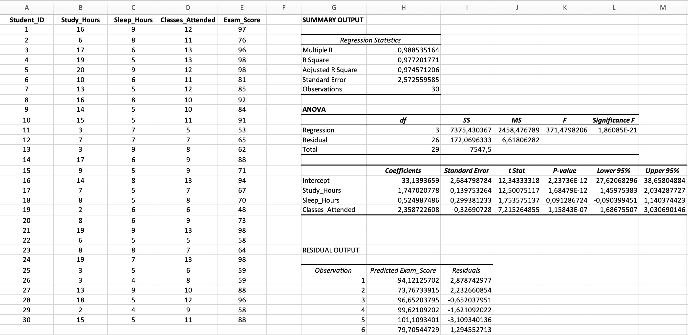
Figure 5: Complete multiple regression output with Regression Statistics, ANOVA, and Coefficients sections
Interpreting Multiple Regression Results
Understanding what each statistic means is critical for your Results chapter. Multiple regression output requires more careful interpretation than simple regression because you're evaluating both the overall model AND individual predictors.
Section 1: Regression Statistics
| Statistic | Example Value | Interpretation |
|---|---|---|
| Multiple R | 0.988 | Correlation between observed Y and predicted Y (always positive) |
| R Square | 0.977 | 97.7% of variance in exam scores is explained by the three predictors combined |
| Adjusted R Square | 0.975 | 97.5% adjusted for number of predictors - use this for multiple regression |
| Standard Error | 2.57 | Average prediction error (in exam score points) |
| Observations | 30 | Sample size |
Table 2: Regression Statistics Output Interpretation
Why Adjusted R² Matters for Multiple Regression
This is crucial: In multiple regression, always report Adjusted R², not just R².
The problem with regular R²: Every time you add a predictor to your model, R² increases - even if that predictor is useless (like shoe size predicting exam scores). R² can never decrease when you add variables.
The solution - Adjusted R²: This statistic penalizes adding unhelpful predictors. It can actually decrease if a new variable doesn't improve prediction enough to justify its inclusion.
When to use which:
- Simple regression (1 predictor): R² and Adjusted R² are nearly identical - use either
- Multiple regression (2+ predictors): Always use Adjusted R² for model evaluation
- Comparing models: If Adjusted R² drops when you add a variable, that variable probably isn't useful
Interpreting R² magnitude: Cohen (1988) suggested that in behavioral research, R² = .02 represents a small effect, R² = .13 a medium effect, and R² = .26 a large effect. An adjusted R² of .975 in our example is exceptionally large, though this teaching dataset was designed for clarity. Real behavioral research typically yields smaller effects (R² = .10 to .30 is common).
Example interpretation: "The three-predictor model explained 97.7% of variance in exam scores (R² = .977, adjusted R² = .975). The minimal difference between R² and adjusted R² suggests all predictors contribute meaningfully to the model."
Section 2: ANOVA Table (Overall Model Significance)
| Source | df | SS | MS | F | Significance F |
|---|---|---|---|---|---|
| Regression | 3 | 2,638.68 | 879.56 | 373.65 | < 0.001 |
| Residual | 26 | 172.07 | 6.62 | - | - |
| Total | 29 | 2,810.75 | - | - | - |
Table 3: ANOVA Table for Multiple Regression Model
Key value: Significance F < 0.001
This tests the null hypothesis that ALL regression coefficients equal zero (i.e., none of the predictors matter).
- If Significance F < 0.05: The overall model is statistically significant - at least one predictor is useful
- If Significance F ≥ 0.05: The model is not significant - the predictors don't predict Y
Important: A significant overall model doesn't mean ALL predictors are significant. You must check each predictor individually in the Coefficients table.
Example interpretation: "The regression model was statistically significant, F(3, 26) = 373.65, p < .001, indicating that the set of predictors (study hours, sleep, and class attendance) significantly predicted exam scores."
Section 3: Coefficients Table (Individual Predictor Significance)
This is where you determine which specific predictors matter - the most important part of multiple regression output.
| Variable | Coefficients (B) | Standard Error | t Stat | P-value | Lower 95% | Upper 95% |
|---|---|---|---|---|---|---|
| Intercept | 33.14 | 2.68 | 12.34 | < 0.001 | 27.63 | 38.65 |
| Study_Hours | 1.75 | 0.14 | 12.50 | < 0.001 | 1.46 | 2.04 |
| Sleep_Hours | 0.52 | 0.30 | 1.75 | 0.092 | -0.09 | 1.14 |
| Classes_Attended | 2.36 | 0.33 | 7.22 | < 0.001 | 1.69 | 3.04 |
Table 4: Regression Coefficients with Individual Predictor Significance
The regression equation:
Which Predictors Are Significant? (Critical Interpretation)
This is where many students make mistakes. You must evaluate each predictor's p-value individually:
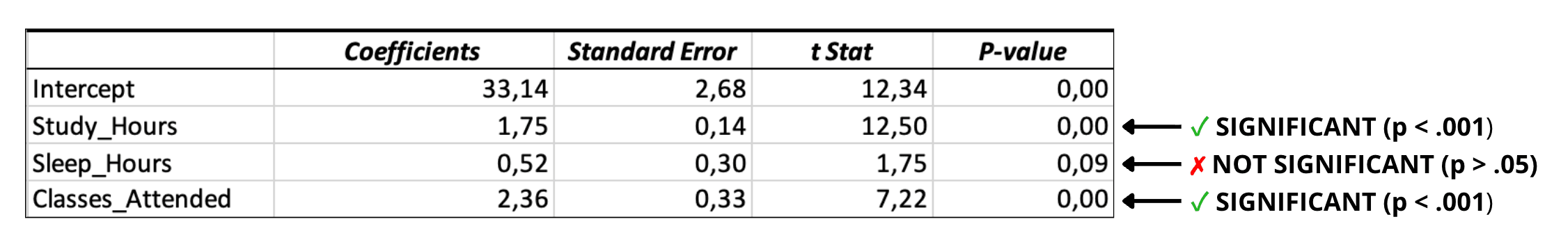
Figure 6: Identifying significant vs. non-significant predictors in the Coefficients table
Interpreting Each Predictor
Study_Hours (p < 0.001) - SIGNIFICANT ✓
- B = 1.75: For each additional hour of study per week, exam scores increase by 1.75 points, holding sleep and attendance constant
- 95% CI [1.46, 2.04]: The true effect is between 1.46 and 2.04 points per hour
- Conclusion: Study hours is a significant unique predictor of exam scores
Sleep_Hours (p = 0.092) - NOT SIGNIFICANT ✗
- B = 0.52: The coefficient suggests 0.52 points per hour of sleep, BUT...
- p = 0.092 > 0.05: This effect is not statistically significant
- 95% CI [-0.09, 1.14]: The interval includes zero, confirming non-significance
- Conclusion: Sleep hours does not significantly predict exam scores after controlling for study hours and attendance
Classes_Attended (p < 0.001) - SIGNIFICANT ✓
Class attendance also emerged as a significant predictor (B = 2.36, 95% CI [1.69, 3.04]). Each additional class attended corresponds to a 2.36-point increase in exam scores when study hours and sleep are held constant. The confidence interval excludes zero, confirming the effect is statistically reliable.
What Does "Not Significant" Mean?
When a predictor is not significant (p ≥ 0.05), it means ONE of these:
-
The variable doesn't actually predict Y - Sleep genuinely doesn't affect exam scores in this population
-
Multicollinearity - Sleep might be correlated with study hours, so when we control for study hours, sleep has no unique contribution left to explain
-
Insufficient power - With a larger sample, the effect might become significant (sample size was only n = 30)
-
True but small effect - The effect exists but is too small to detect with this sample
How to report non-significant predictors: Don't hide them! Report all predictors you tested, including non-significant ones. This is methodologically honest and helps readers understand your full model.
Comparing Predictor Importance
A natural question: "Which predictor matters most?" This requires standardized coefficients.
Standardized vs Unstandardized Coefficients
Excel gives you unstandardized coefficients (B) which are in the original units of each variable:
- Study hours: 1.75 points per hour
- Classes: 2.36 points per class
You can't directly compare 1.75 vs 2.36 because the scales are different (hours vs classes attended).
Calculating Standardized Coefficients (β) in Excel
To compare predictor importance, calculate standardized coefficients manually:
Steps:
- Calculate the standard deviation of each predictor using
=STDEV.S(range) - Calculate the standard deviation of Y (exam scores)
- Multiply each unstandardized B by (SD_X / SD_Y)
Example calculations:
-
SD(Study_Hours) = 5.73, SD(Exam_Score) = 9.65
-
β(Study_Hours) = 1.75 × (5.73 / 9.65) = 1.04
-
SD(Classes_Attended) = 2.56
-
β(Classes_Attended) = 2.36 × (2.56 / 9.65) = 0.63
Interpretation: Study hours (β = 1.04) has a larger standardized effect than class attendance (β = 0.63), making it the stronger predictor of exam performance.
Note: For formal thesis research requiring standardized coefficients, SPSS provides them automatically in the "Standardized Coefficients Beta" column. If calculating manually in Excel, verify your results by confirming that predictors with stronger correlations with Y also have larger standardized coefficients. If your rankings don't match, check your standard deviation calculations.
Detecting Multicollinearity in Excel
Multicollinearity is THE critical issue unique to multiple regression that Excel tutorials often ignore. It occurs when your predictor variables are highly correlated with each other - and it can seriously distort your results.
Why Multicollinearity is a Problem
When predictors are highly correlated:
- Coefficients become unstable - small data changes cause large coefficient swings
- Standard errors inflate - making significant predictors appear non-significant
- Signs may flip - a predictor that should be positive becomes negative
- You can't tell which predictor matters - their effects are confounded
Example: If study hours and library hours are highly correlated (r = 0.95), the model can't separate their effects. One might appear significant while the other doesn't, but swapping which one you include would reverse the results.
How to Check for Multicollinearity in Excel
Excel cannot calculate VIF (Variance Inflation Factor), but you CAN detect multicollinearity using a correlation matrix:
Step 1: Create a Correlation Matrix
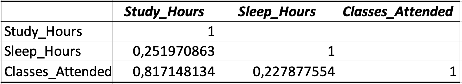
Figure 7: Correlation matrix of predictor variables - most correlations are low, with one borderline value (r = 0.82)
- Click Data → Data Analysis → Correlation
- Input Range: Select only your predictor columns (X variables), not Y
- Check Labels in first row
- Click OK
Step 2: Interpret the Correlation Matrix
| Study_Hours | Sleep_Hours | Classes_Attended | |
|---|---|---|---|
| Study_Hours | 1.00 | 0.25 | 0.82 |
| Sleep_Hours | 0.25 | 1.00 | 0.23 |
| Classes_Attended | 0.82 | 0.23 | 1.00 |
Table 5: Correlation Matrix of Predictor Variables
Decision rules:
- r < 0.70: No concern - predictors are sufficiently independent
- 0.70 ≤ r < 0.80: Moderate concern - monitor but usually acceptable
- r ≥ 0.80: High concern - multicollinearity likely problematic
- r ≥ 0.90: Severe concern - consider removing one predictor
In our example: Most correlations are low (0.23–0.25). The correlation between Study_Hours and Classes_Attended (r = 0.82) is at the 0.80 threshold but acceptable for this teaching example. In thesis research, you might consider whether these variables measure overlapping constructs - students who study more may also attend more classes. Despite this borderline correlation, our regression coefficients remain interpretable and both predictors are significant.
Warning Signs of Multicollinearity in Output
Even without a correlation matrix, watch for these red flags in your regression output:
- Very large standard errors for coefficients (relative to the coefficient size)
- Coefficients with unexpected signs (positive should be negative, or vice versa)
- Significant overall model but no significant individual predictors
- Coefficients that change dramatically when you add/remove a predictor
What to Do If You Have Multicollinearity
If correlations between predictors exceed 0.80:
- Remove one of the correlated predictors - Keep the one most theoretically important
- Combine correlated predictors - Create a composite score (e.g., average of study hours + library hours)
- Use Principal Component Analysis - Requires SPSS or R
- Center your variables - Subtract the mean from each predictor (helps with interaction terms)
- Report it as a limitation - If you can't fix it, acknowledge it
For thesis committees requiring VIF: You'll need SPSS or R. VIF > 5 indicates problems; VIF > 10 is severe. Excel cannot calculate VIF.
Checking Multiple Regression Assumptions
Multiple regression has five assumptions - one more than simple regression. Violating assumptions can invalidate your p-values and conclusions.
The Five Assumptions
- Linearity - Relationship between each X and Y is linear
- Independence - Observations are independent of each other
- Normality of Residuals - Prediction errors are normally distributed
- Homoscedasticity - Residuals have constant variance
- No Multicollinearity - Predictors are not highly correlated (UNIQUE to multiple regression)
Why assumptions matter: Each violation causes specific problems. Non-linearity biases coefficient estimates (your B values will be wrong). Heteroscedasticity inflates standard errors, making genuinely significant effects appear non-significant. Non-normality of residuals affects the accuracy of confidence intervals and p-values, particularly in smaller samples. Multicollinearity makes individual coefficients uninterpretable because the model cannot separate the effects of correlated predictors.
Assumption 1: Linearity
How to check: Create scatter plots of each X vs Y individually.
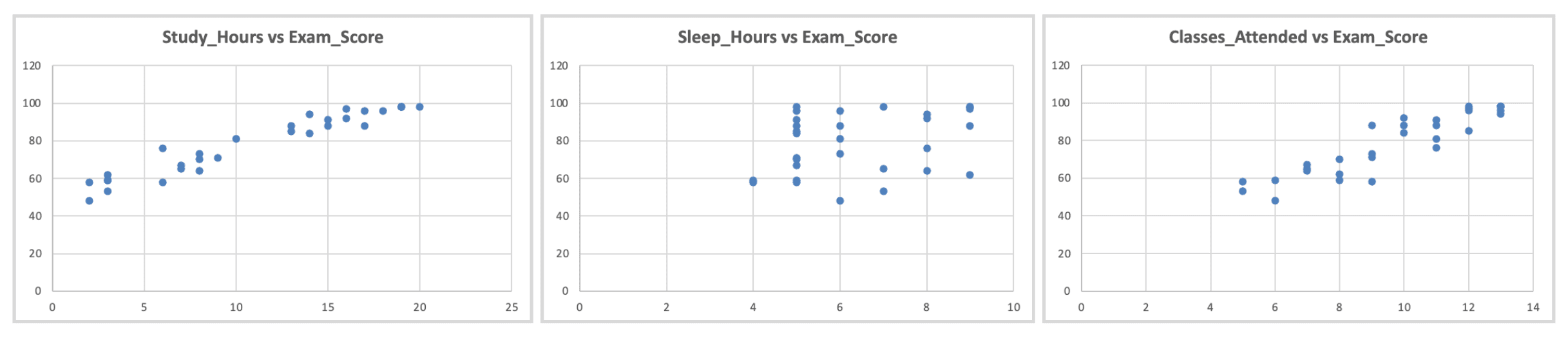
Figure 8: Linearity check - scatter plots of each predictor vs. outcome showing approximately linear relationships
What to look for: Roughly linear patterns (not curved, U-shaped, or exponential)
Assumption 2: Independence
This is a research design issue, not something you test statistically.
Independent: Each observation is a different person, measured once Not independent: Same people measured multiple times, or people nested in groups (classrooms, families)
Excel cannot test this - ensure independence through your research design.
Assumption 3: Normality of Residuals
How to check: Create a histogram of residuals.
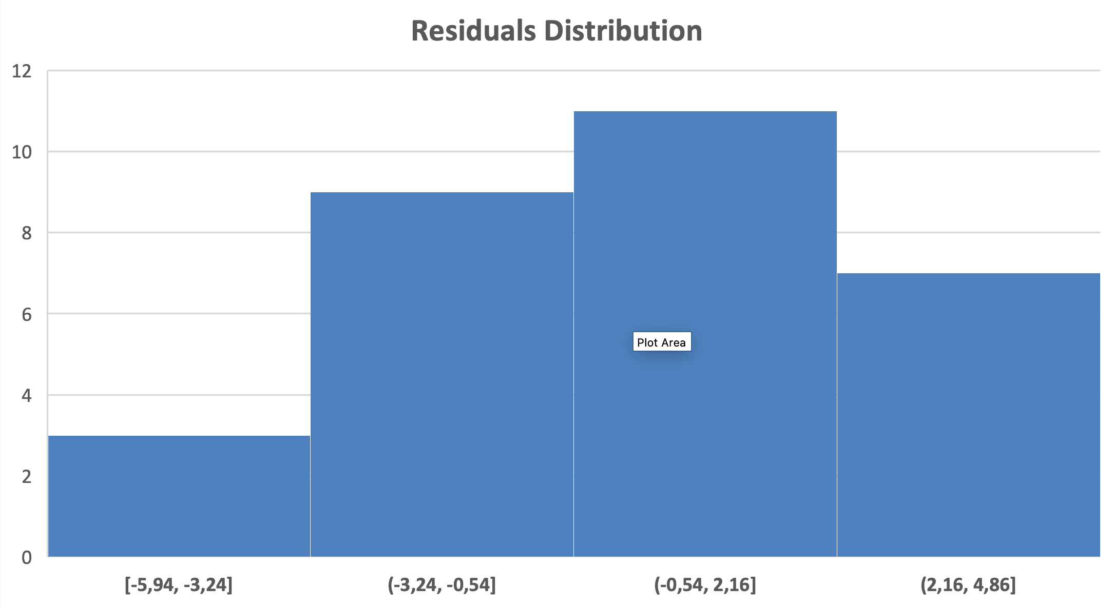
Figure 9: Normality check - histogram of residuals shows approximately normal distribution
Steps:
- Check Residuals box in the regression dialog
- Find the Residuals column in output
- Create histogram: Select residuals → Insert → Histogram (for detailed histogram creation, see our descriptive statistics guide)
What to look for: Bell-shaped, symmetric distribution centered around zero.
Assumption 4: Homoscedasticity (Constant Variance)
How to check: Plot residuals vs. predicted (fitted) values.
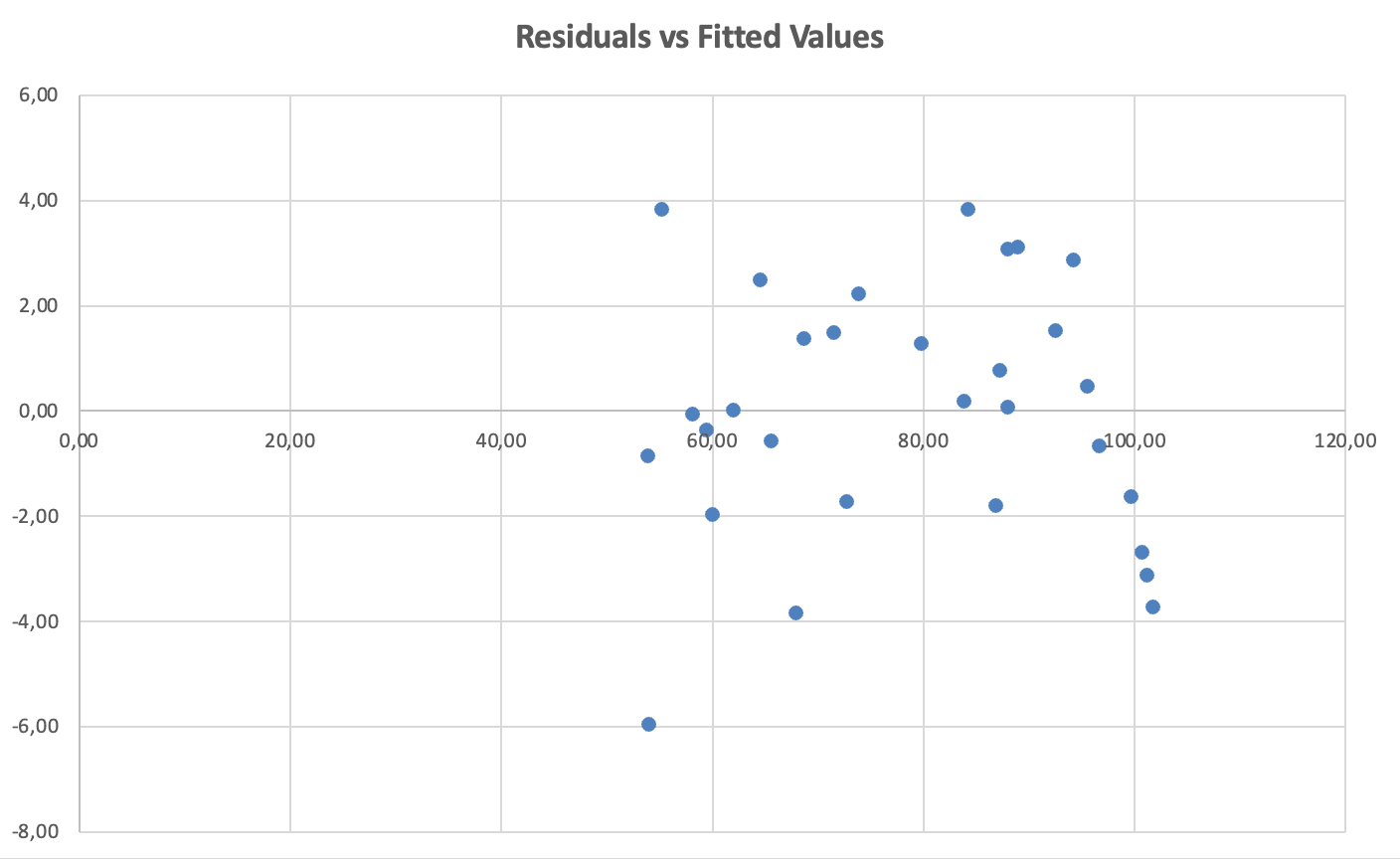
Figure 10: Homoscedasticity check - residuals vs. fitted values show constant spread (no funnel pattern)
What to look for: Random scatter around zero with roughly constant spread across all fitted values. Violation: Funnel or cone shape (spread increases or decreases).
Assumption 5: No Multicollinearity (UNIQUE to Multiple Regression)
How to check: Correlation matrix of predictors (covered in previous section).
Rule: Correlations between predictors should be below 0.80.
Reporting Assumptions in Your Thesis
In Methods section:
Prior to analysis, assumptions for multiple linear regression were evaluated. Scatter plots indicated linear relationships between each predictor and the outcome variable. The Durbin-Watson statistic was not available in Excel; however, observations were independent by research design (different students with single measurements). Histograms of residuals showed approximately normal distribution, and residual plots indicated constant variance (homoscedasticity). Multicollinearity was assessed using a correlation matrix of predictor variables; most correlations were low (r = 0.23–0.25), though Study_Hours and Classes_Attended showed a borderline correlation (r = 0.82) that was monitored but did not substantially affect coefficient interpretability.
How to Report Multiple Regression in APA 7th Edition Format
Your thesis committee expects multiple regression results reported with specific elements. Here's the complete format.
APA Results Section Template
Paragraph format:
A multiple linear regression was conducted to examine whether study hours, sleep hours, and class attendance predicted final exam scores. Preliminary analyses confirmed that assumptions of linearity, independence, normality of residuals, homoscedasticity, and absence of multicollinearity were met.
The multiple regression model statistically significantly predicted exam scores, F(3, 26) = 373.65, p < .001, R² = .98, adjusted R² = .97. The three predictors together explained 97.7% of variance in exam scores. Regression coefficients are presented in Table [X].
Study hours significantly predicted exam scores (B = 1.75, 95% CI [1.46, 2.04], p < .001), as did class attendance (B = 2.36, 95% CI [1.69, 3.04], p < .001). Sleep hours was not a statistically significant predictor (B = 0.52, 95% CI [-0.09, 1.14], p = .092). For each additional hour of weekly study, exam scores increased by 1.75 points, controlling for sleep and attendance. Each additional class attended was associated with a 2.36-point increase in exam scores, controlling for other predictors.
APA Regression Table Format
Table [X]
Multiple Linear Regression Predicting Exam Scores
| Variable | B | SE | β | t | p | 95% CI |
|---|---|---|---|---|---|---|
| Intercept | 33.14 | 2.68 | — | 12.34 | < .001 | [27.63, 38.65] |
| Study Hours | 1.75 | 0.14 | 1.04 | 12.50 | < .001 | [1.46, 2.04] |
| Sleep Hours | 0.52 | 0.30 | .09 | 1.75 | .092 | [-0.09, 1.14] |
| Classes Attended | 2.36 | 0.33 | .63 | 7.22 | < .001 | [1.69, 3.04] |
Table 6: Multiple Linear Regression Predicting Exam Scores from Study Hours, Sleep Hours, and Class Attendance
Note. n = 30. R² = .98, adjusted R² = .97, F(3, 26) = 373.65, p < .001. B = unstandardized coefficient. SE = standard error. β = standardized coefficient. CI = confidence interval.
Reporting Checklist for Multiple Regression
Include ALL of these elements:
In-text (Results paragraph):
- Analysis type ("A multiple linear regression was conducted...")
- Variables tested (all predictors and outcome)
- Assumption checking statement
- Overall model significance: F(df_regression, df_residual) = F-value, p-value
- R² AND adjusted R² with interpretation
- For EACH predictor: B value, 95% CI, and p-value
- Clear statement of which predictors were/weren't significant
- Interpretation of significant coefficients with direction
In table:
- Table number and italicized title
- All predictors including intercept
- B (unstandardized coefficients)
- SE (standard errors)
- β (standardized coefficients) if calculated
- t-statistics
- p-values -95% confidence intervals
- Table note with n, R², adjusted R², F-statistic
Common Mistakes in Multiple Regression
Avoid these frequent errors that can compromise your thesis research:
1. Reporting R² Instead of Adjusted R²
Mistake: "The model explained 97.5% of variance (R² = .975)"
Why it's wrong: R² always increases with more predictors, even useless ones. Adjusted R² corrects for this.
How to fix: Report adjusted R² as your primary effect size, or report both: "R² = .972, adjusted R² = .969"
2. Ignoring Multicollinearity
Mistake: Adding highly correlated predictors without checking.
Why it's wrong: Coefficients become unstable, standard errors inflate, and you can't interpret which predictor matters.
How to fix: Always create correlation matrix of predictors before running regression. Remove or combine variables with r > 0.80.
3. Removing Non-Significant Predictors Without Justification
Mistake: "Sleep wasn't significant, so I removed it and reran the analysis."
Why it's wrong: Removing variables changes the meaning of other coefficients. Selective removal can lead to biased results.
How to fix: Keep all theoretically relevant predictors. Report non-significant ones as non-significant. Only remove if you have strong theoretical reasons AND report that you did so.
4. Interpreting Coefficients as "Most Important"
Mistake: "Study hours (B = 2.15) is more important than attendance (B = 1.85) because 2.15 > 1.85."
Why it's wrong: Unstandardized coefficients depend on the scale of each variable. You're comparing hours to classes - different units.
How to fix: Calculate and compare standardized coefficients (β) for importance comparisons.
5. Claiming Causation from Regression
Mistake: "Studying more CAUSES higher exam scores."
Why it's wrong: Regression shows prediction and association, not causation. Causation requires experimental design with random assignment.
How to fix: Use careful language - "predicted," "associated with," "related to" rather than "caused," "led to," "resulted in."
6. Not Checking Assumptions
Mistake: Running regression without verifying linearity, normality, homoscedasticity, and multicollinearity.
Why it's wrong: Violated assumptions lead to biased coefficients and invalid p-values.
How to fix: Always check all five assumptions before finalizing results. Report assumption checking in Methods.
7. Using Too Many Predictors for Sample Size
Mistake: Including 10 predictors with only 50 observations.
Why it's wrong: Overfitting occurs when the model fits your sample but fails to generalize. The minimum requirement is n ≥ 50 + 8k.
How to fix: Follow sample size guidelines. For 10 predictors, you need at least n = 130 observations. If missing data has reduced your available sample, address this first. See how to handle missing data for strategies to maximize your usable sample size.
What Excel Cannot Do: Limitations for Thesis Research
Excel's Analysis ToolPak handles standard multiple linear regression well, but has significant limitations for advanced techniques. Understanding these helps you choose the right software.
Regression Types Requiring SPSS or R
| Technique | What It Does | Excel? | Use Instead |
|---|---|---|---|
| Logistic Regression | Predicts binary outcomes (yes/no) | No | SPSS, R |
| Stepwise Regression | Automatic variable selection | No | SPSS, R |
| Hierarchical Regression | Adds predictors in blocks | No | SPSS |
| Moderation Analysis | Tests interaction effects | No | SPSS PROCESS |
| Mediation Analysis | Tests indirect effects | No | SPSS PROCESS |
| VIF Calculation | Formal multicollinearity test | No | SPSS, R |
| Durbin-Watson | Tests autocorrelation | No | SPSS, R |
| Polynomial Regression | Curved relationships | Yes (manual) | SPSS, R |
| Multiple Linear Regression | 2+ continuous predictors | Yes | All software |
Table 7: Excel Regression Capabilities vs. Statistical Software Requirements
When to Use Excel vs SPSS/R
Use Excel when:
- Standard multiple linear regression only
- Continuous outcome variable
- You don't need VIF (correlation matrix is sufficient)
- Committee accepts Excel output
- Learning regression before advanced methods
Use SPSS/R when:
- Binary/categorical outcomes (logistic regression)
- Need stepwise or hierarchical regression
- Testing moderation or mediation
- Committee requires VIF, Durbin-Watson
- Publishing in journals requiring SPSS/R output
Key takeaway: Excel is excellent for learning multiple regression and for basic thesis analyses. For advanced techniques or formal multicollinearity testing, you'll need SPSS or R. Check with your advisor about software requirements.
Frequently Asked Questions
Committee Questions You Should Be Ready to Answer
Thesis committees commonly ask these questions about multiple regression analyses. Preparing answers in advance demonstrates statistical competence and strengthens your defense.
"Why did you include these specific predictors?"
Be prepared to justify each variable based on theory and prior research, not just statistical convenience. Cite literature showing why each predictor should logically relate to your outcome. Committees are skeptical of "data dredging" where predictors were included simply because data was available.
"Did you check for multicollinearity?"
Show your correlation matrix and explain that all predictor correlations were below 0.80 (or whatever your threshold was). If asked about VIF and you used Excel, explain that while Excel cannot calculate VIF directly, the correlation matrix method identifies problematic multicollinearity. Acknowledge that SPSS or R would be needed for formal VIF testing.
"Why is [variable] not significant?"
A non-significant predictor does not mean the variable is unimportant. Explain that when controlling for other predictors, this variable's unique contribution was not statistically distinguishable from zero. Possible reasons include: overlap with other predictors (shared variance), insufficient sample size to detect a small effect, or genuinely no unique relationship after controlling for confounders.
"What's the practical significance of these results?"
Statistical significance is not the same as practical importance. Be ready to explain what a coefficient means in real terms. For example: "Each additional study hour is associated with a 1.75-point increase in exam scores. Over a semester, a student who studies 10 hours more per week than average could expect roughly 17.5 additional points, potentially the difference between a B and an A."
"Why didn't you use SPSS or R?"
If asked, explain that Excel's Analysis ToolPak handles standard multiple linear regression adequately for your research design. Acknowledge Excel's limitations (no VIF, no stepwise regression, no logistic regression) and explain why these weren't required for your specific analysis. If your committee strongly prefers SPSS output, offer to replicate the analysis in SPSS for the final submission.
Next Steps: Applying Multiple Regression to Your Thesis
You now have a complete framework for conducting multiple linear regression in Excel - from understanding when to use it, through running the analysis, to interpreting results and reporting in APA format. The key to success is not just running the analysis, but understanding what each output means and checking that your data meets the assumptions.
Before finalizing your analysis:
-
Check multicollinearity first - Create a correlation matrix of predictors before running regression. Correlations > 0.80 require action.
-
Verify all five assumptions - Linearity, independence, normality of residuals, homoscedasticity, AND no multicollinearity.
-
Use adjusted R² - This is the appropriate effect size for multiple regression, not regular R².
-
Report ALL predictors - Include non-significant predictors in your Results table. Don't selectively remove variables without strong justification.
-
Know Excel's limitations - If you need VIF, stepwise regression, or logistic regression, you'll need SPSS or R.
Related guides to continue your learning:
- Prerequisite: Simple Linear Regression in Excel - Review if concepts here were unclear
- Correlation: Pearson Correlation Coefficient - For checking multicollinearity
- Effect Size: How to Calculate Effect Size - For interpreting practical significance
- Reporting: Report Descriptive Statistics in APA - For complete Results chapters
- Group Differences: ANOVA in Excel - When predictors are categorical groups
References
American Psychological Association. (2020). Publication manual of the American Psychological Association (7th ed.). https://doi.org/10.1037/0000165-000
Cohen, J. (1988). Statistical power analysis for the behavioral sciences (2nd ed.). Lawrence Erlbaum Associates.
Green, S. B. (1991). How many subjects does it take to do a regression analysis? Multivariate Behavioral Research, 26(3), 499–510. https://doi.org/10.1207/s15327906mbr2603_7
Hair, J. F., Black, W. C., Babin, B. J., & Anderson, R. E. (2019). Multivariate data analysis (8th ed.). Cengage Learning.
Tabachnick, B. G., & Fidell, L. S. (2019). Using multivariate statistics (7th ed.). Pearson.