You ran a t-test or ANOVA in Excel for your dissertation. The p-value shows statistical significance. Your committee asks: "What's the effect size?"
Statistical significance tells you a difference exists. Effect size tells you if that difference matters. A p-value of .001 with 10,000 participants might represent a trivial difference that has no practical value. An effect size shows the magnitude of your findings independent of sample size.
This guide shows you how to calculate Cohen's d for t-tests and eta squared for ANOVA in Excel. You will learn the exact formulas, interpretation guidelines by discipline, and how to report effect sizes in APA format for your thesis results chapter.
Why Effect Size Matters for Your Dissertation
Your dissertation committee evaluates both statistical and practical significance. A statistically significant result (p < .05) only indicates a difference probably exists in the population. It does not indicate whether that difference is large enough to matter.
Effect size provides three critical pieces of information for your thesis:
Practical significance. A study with 5,000 participants might show that Method A produces test scores 2 points higher than Method B (p < .001). Statistical significance is clear, but is a 2-point difference on a 100-point scale meaningful? Cohen's d quantifies this.
Comparability across studies. Your literature review compares studies with different sample sizes. Effect sizes standardize findings so you can compare a study with n of 30 to one with n of 3,000. P-values cannot do this.
Research impact. Journal editors and thesis committees want evidence your findings matter beyond your sample. Small effect sizes (even if significant) suggest limited real-world application. Large effect sizes indicate your intervention or finding has substantial practical value.
Most APA-style thesis committees now require effect size reporting for all inferential tests. The 7th edition of the APA Publication Manual explicitly recommends reporting effect sizes alongside p-values in results sections.
When to Use Cohen's d vs Eta Squared
Your statistical test determines which effect size measure you calculate.
| Statistical Test | Effect Size Measure | What It Measures | Interpretation Scale |
|---|---|---|---|
| Independent samples t-test | Cohen's d | Standardized difference between two group means | 0.2 small, 0.5 medium, 0.8 large |
| Paired samples t-test | Cohen's d | Standardized difference between paired observations | 0.2 small, 0.5 medium, 0.8 large |
| One-Way ANOVA | Eta squared (η²) or Omega squared (ω²) | Proportion of variance in DV explained by IV | 0.01 small, 0.06 medium, 0.14 large |
| Two-Way ANOVA | Partial eta squared (η²p) | Variance explained by one factor controlling for others | 0.01 small, 0.06 medium, 0.14 large |
Table 1: Effect size measures for common statistical tests used in dissertations
If you compared two groups (control vs experimental, pre vs post, male vs female), use Cohen's d. If you compared three or more groups (low/medium/high, multiple treatment conditions), use eta squared or omega squared from your ANOVA output.
Both measures answer the same fundamental question: How big is this effect? They use different scales because they measure different things. Cohen's d expresses effect in standard deviation units. Eta squared expresses effect as proportion of variance explained (like R² in regression).
How to Calculate Cohen's d in Excel
Cohen's d measures the standardized difference between two group means. This section shows you the step-by-step calculation using Excel formulas.
Understanding the Cohen's d Formula
The formula for Cohen's d is:
d equals (M₁ minus M₂) divided by SDpooled
Where:
- M₁ equals Mean of Group 1
- M₂ equals Mean of Group 2
- SDpooled equals Pooled standard deviation of both groups
The pooled standard deviation formula is:
SDpooled equals √[((n₁-1) × SD₁² + (n₂-1) × SD₂²) / (n₁ + n₂ - 2)]
Where:
- n₁, n₂ equals Sample sizes for groups 1 and 2
- SD₁, SD₂ equals Standard deviations for groups 1 and 2 (see our guide on how to calculate standard deviation in Excel if you need to compute these first)
Step-by-Step Calculation in Excel
Example scenario: You tested a new teaching method on student exam scores. The control group (n of 25) had M of 72.4, SD of 8.3. The experimental group (n of 28) had M of 79.6, SD of 7.9. Calculate Cohen's d.
Note on Decimal Separators: Depending on your regional settings, Excel may display decimals with a period (72.4) or a comma (72,4). Both are correct. It's just a locale setting. If your Excel shows commas but you want periods (or vice versa), go to:
- Windows: File → Options → Advanced → Editing options → uncheck "Use system separators" and set your preferred Decimal separator
- Mac: System Preferences → Language & Region → Advanced → Number separators
The formulas in this guide use semicolons (;) or commas (,) as argument separators depending on your locale. If a formula doesn't work, try swapping commas for semicolons in the formula arguments.
Step 1: Set up your data in Excel
Create a table with your descriptive statistics:
| Statistic | Control Group | Experimental Group |
|---|---|---|
| Sample size (n) | 25 | 28 |
| Mean (M) | 72.4 | 79.6 |
| Standard deviation (SD) | 8.3 | 7.9 |
Table 2: Descriptive statistics for the control and experimental groups
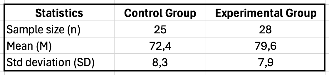
Figure 1: Excel table setup for Cohen's d calculation showing sample size, mean, and standard deviation for control and experimental groups
Step 2: Calculate the pooled standard deviation
In a new cell (e.g., B7), enter this formula:
=SQRT(((B2-1)*B4^2 + (C2-1)*C4^2)/(B2+C2-2))
This calculates: √[((25-1) × 8.3² + (28-1) × 7.9²) / (25 + 28 - 2)]
Result: SDpooled equals 8.09
Step 3: Calculate Cohen's d
In cell B8, enter:
=ABS(B3-C3)/B7
This calculates: |72.4 - 79.6| / 8.09
Result: d equals 0.89
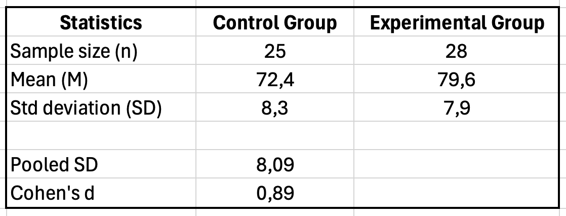
Figure 2: Excel Cohen's d calculation showing pooled standard deviation of 8.09 and Cohen's d result of 0.89
Alternative: Using Descriptive Statistics Directly
If you already ran a t-test and have your descriptive statistics, you can create a simple Cohen's d calculator in Excel:
| Cell | Label | Formula/Value | Description |
|---|---|---|---|
| A1 | Group 1 Mean | 72.4 | Enter your M₁ value |
| A2 | Group 2 Mean | 79.6 | Enter your M₂ value |
| A3 | Group 1 SD | 8.3 | Enter your SD₁ value |
| A4 | Group 2 SD | 7.9 | Enter your SD₂ value |
| A5 | Group 1 n | 25 | Enter your n₁ value |
| A6 | Group 2 n | 28 | Enter your n₂ value |
| A7 | Pooled SD | =SQRT(((A5-1)*A3^2+(A6-1)*A4^2)/(A5+A6-2)) | Calculated automatically |
| A8 | Cohen's d | =ABS(A1-A2)/A7 | Your effect size |
Table 3: Excel calculator template for Cohen's d (save this as a reusable template)
Save this template for quick Cohen's d calculations throughout your dissertation analysis.
How to Calculate Cohen's d for Paired Samples in Excel
The formula above works for independent samples (two different groups). If you compared the same participants at two time points (pre-test vs post-test, before vs after intervention), you need a different calculation.
Understanding the Paired Samples Formula
For paired samples, Cohen's d uses the mean difference and standard deviation of the differences:
d = Mean of differences / SD of differences
This is sometimes called dz (d-sub-z) in the literature. It accounts for the fact that paired observations are correlated.
Step-by-Step Calculation in Excel
Example scenario: You measured anxiety scores for 30 participants before and after a mindfulness intervention. You need to calculate the effect size for your pre-post comparison.
Step 1: Calculate the difference for each participant
If your pre-test scores are in column A (A2:A31) and post-test scores are in column B (B2:B31), create a difference column in column C:
=B2-A2
Copy this formula down for all 30 participants.
Step 2: Calculate the mean of differences
In a cell below your data (e.g., C33):
=AVERAGE(C2:C31)
Example result: Mean difference = -8.4 (negative indicates anxiety decreased)
Step 3: Calculate the standard deviation of differences
In cell C34:
=STDEV.S(C2:C31)
Example result: SD of differences = 6.2
Step 4: Calculate Cohen's d
In cell C35:
=ABS(C33)/C34
This calculates: |−8.4| / 6.2 = 1.35
Result: d = 1.35 (a very large effect)
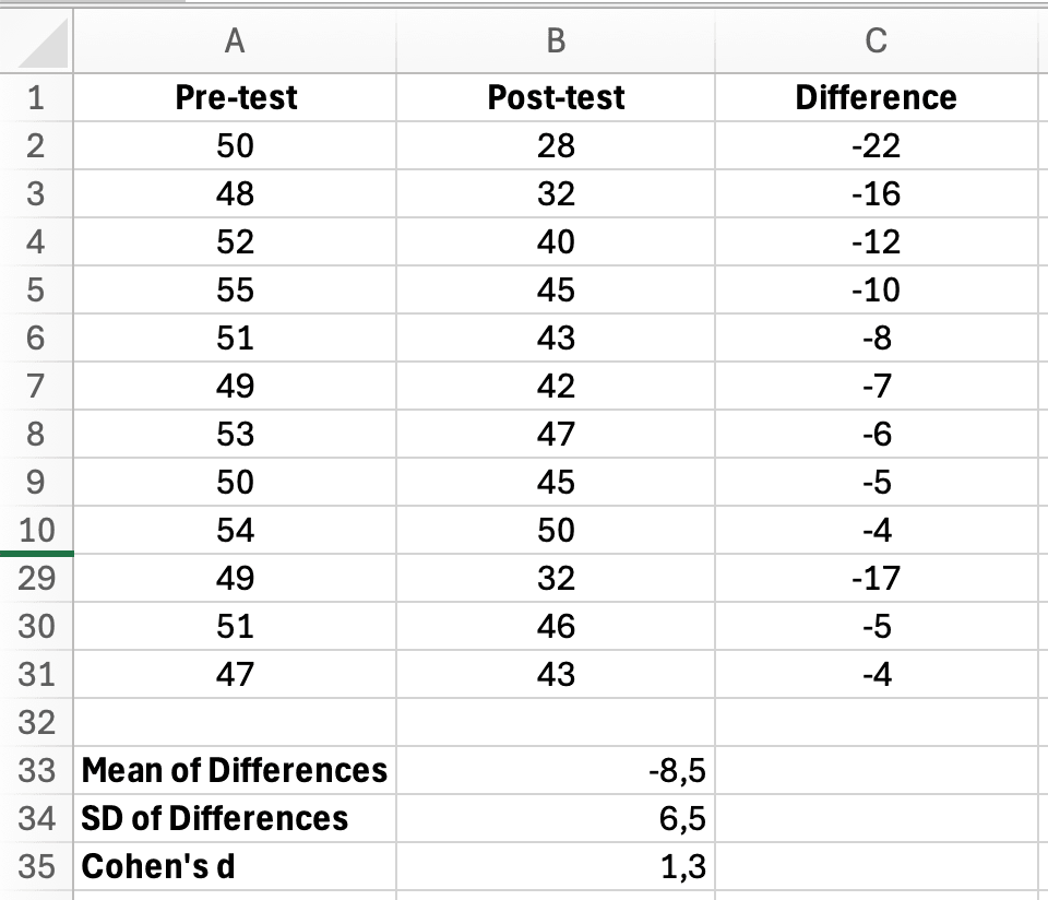
Figure 3: Excel paired samples Cohen's d calculation showing Pre-test, Post-test, Difference columns with mean of differences, SD, and Cohen's d result of 1.3
Paired Samples Calculator Template
Create this reusable template for paired samples effect sizes:
| Cell | Label | Formula/Value | Description |
|---|---|---|---|
| A1 | Mean of Differences | =AVERAGE(difference_range) | Average pre-post change |
| A2 | SD of Differences | =STDEV.S(difference_range) | Variability in change scores |
| A3 | Cohen's d (paired) | =ABS(A1)/A2 | Your effect size |
Table 4: Excel calculator template for paired samples Cohen's d (pre-post designs)
Important Note: Paired vs Independent Effect Sizes
Effect sizes from paired designs (dz) tend to be larger than independent designs because the SD of differences is typically smaller than the pooled SD of raw scores. This is not an error. It reflects the increased precision of within-subjects comparisons.
When comparing your effect size to published literature, verify whether the studies used paired or independent designs. If you need to compare across study types, some researchers calculate Cohen's d using the average of pre and post standard deviations (called dav) instead of the SD of differences.
How to Calculate Eta Squared in Excel
Eta squared (η²) measures the proportion of total variance in your dependent variable explained by your independent variable in ANOVA. This section shows you how to extract and calculate it from Excel's ANOVA output.
Understanding the Eta Squared Formula
The formula for eta squared is:
η² equals SSBetween divided by SSTotal
Where:
- SSBetween equals Sum of Squares Between Groups (variation explained by your grouping variable)
- SSTotal equals Total Sum of Squares (total variation in your data)
Eta squared tells you what percentage of the variance in your dependent variable is attributable to your independent variable. An η² of 0.25 means your grouping variable explains 25% of the variance in outcomes.
Step-by-Step Calculation from ANOVA Output
Example scenario: You compared student engagement scores across three teaching methods (traditional, blended, online). You ran One-Way ANOVA in Excel and need to calculate effect size.
Step 1: Run One-Way ANOVA in Excel
First, run your ANOVA using Data Analysis ToolPak (if you haven't enabled it yet, see our guide on how to add Data Analysis in Excel). For detailed instructions on running ANOVA, see our complete guide on how to calculate ANOVA in Excel.
- Click Data > Data Analysis > Anova: Single Factor
- Select your data range (three groups of engagement scores)
- Check "Labels in First Row" if applicable
- Click OK
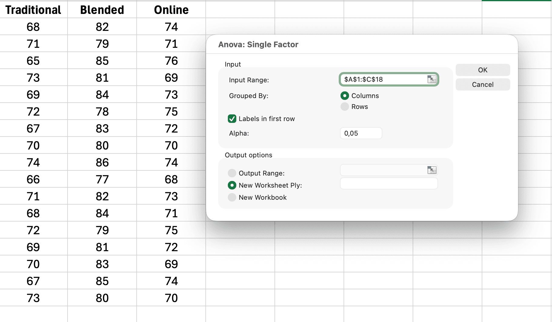
Figure 4: Excel Data Analysis ANOVA Single Factor dialog box showing input range, labels in first row checked, and output options
Step 2: Locate the Sum of Squares values
Excel's ANOVA output table looks like this:
| Source of Variation | SS | df | MS | F | P-value |
|---|---|---|---|---|---|
| Between Groups | 245.6 | 2 | 122.8 | 8.34 | 0.001 |
| Within Groups | 278.2 | 47 | 5.92 | ||
| Total | 523.8 | 49 |
Table 5: Example One-Way ANOVA output from Excel (engagement scores by teaching method)
You need two values:
- SS Between Groups equals 245.6 (variation explained by teaching method)
- SS Total equals 523.8 (total variation in engagement scores)
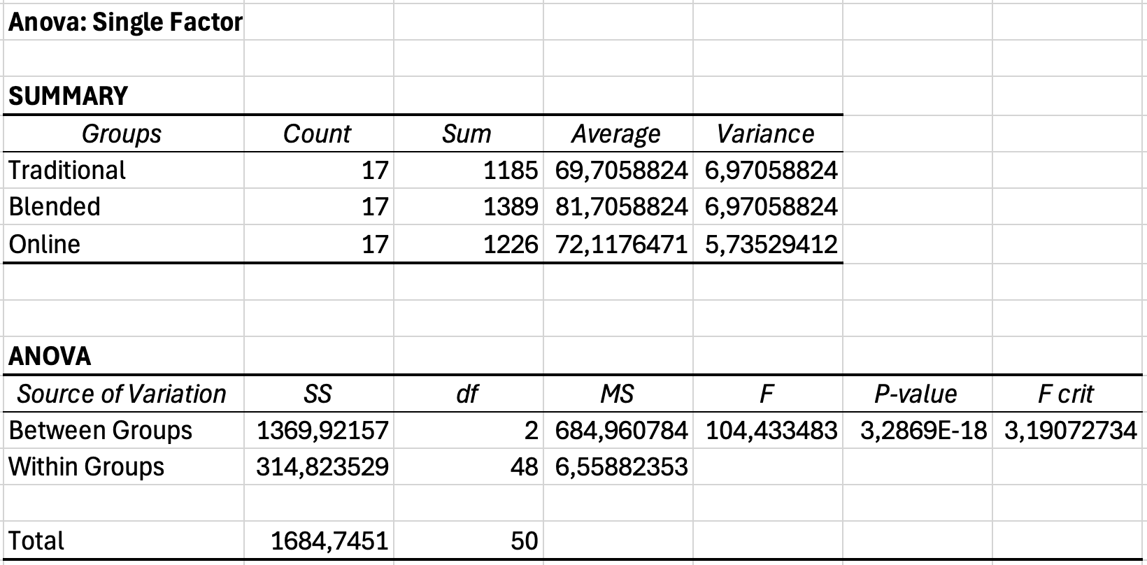
Figure 5: Excel ANOVA output table showing Sum of Squares Between Groups and Total values needed for eta squared calculation
Step 3: Calculate eta squared
In a cell below your ANOVA table, enter:
=B10/B12
(Adjust cell references to match where your SS Between and SS Total appear)
This calculates: 245.6 divided by 523.8 equals 0.469
Step 4: Convert to percentage (optional)
To express as percentage of variance explained:
=B10/B12*100
Result: η² equals 0.469 or 46.9% of variance explained
Creating an Eta Squared Calculator in Excel
For quick calculations, create this simple template next to your ANOVA output:
| Cell | Label | Formula/Value |
|---|---|---|
| D1 | SS Between | =B10 |
| D2 | SS Total | =B12 |
| D3 | Eta Squared (η²) | =D1/D2 |
| D4 | % Variance Explained | =D3*100 |
Table 6: Eta squared calculator template for Excel ANOVA results
This template automatically updates when you run new ANOVA analyses.
Interpreting Effect Sizes for Your Dissertation
Calculating effect size is only the first step. Your thesis committee expects you to interpret whether your effect is small, medium, or large, and what that means for your research question.
Cohen's d Interpretation Guidelines
Jacob Cohen (1988) proposed these benchmarks for behavioral science research:
| Cohen's d Value | Effect Size | Percentile Standing | Overlap Between Distributions |
|---|---|---|---|
| 0.2 | Small | 58th percentile | 85% overlap |
| 0.5 | Medium | 69th percentile | 67% overlap |
| 0.8 | Large | 79th percentile | 53% overlap |
| 1.0 | Very large | 84th percentile | 45% overlap |
Table 7: Cohen's d interpretation with practical meaning (percentile equals where average treatment person ranks in control group)
Practical interpretation example: If your intervention produces d of 0.8, the average person in the treatment group scores at the 79th percentile of the control group. This means 79% of the control group scored lower than the average treatment participant.
Eta Squared Interpretation Guidelines
For ANOVA effect sizes, Cohen suggested:
- η² of 0.01 (1% variance explained) equals Small effect
- η² of 0.06 (6% variance explained) equals Medium effect
- η² of 0.14 (14% variance explained) equals Large effect
Example interpretation: Your teaching method ANOVA produced η² of 0.47 (47% variance explained). This is a very large effect. Teaching method explains nearly half of the variation in student engagement. The remaining 53% is due to individual differences, measurement error, and other unmeasured factors.
Discipline-Specific Considerations
Cohen's guidelines are not universal. Effect size norms vary by field:
Education research: Average d of 0.4 for instructional interventions. Effects of d of 0.2 are common and still practically significant for classroom implementation.
Clinical psychology: Treatment effects of d in range 0.5-0.8 are typical. Smaller effects (d in range 0.2-0.4) may still be clinically meaningful for chronic conditions.
Medicine and public health: Even d of 0.1 can represent important differences when interventions affect mortality or disease incidence. Statistical significance matters more than effect size magnitude.
Experimental psychology: Laboratory studies often show large effects (d greater than 1.0) under controlled conditions. Field studies typically show smaller effects (d in range 0.3-0.5).
Business and management: Effects of d in range 0.3-0.5 are common for organizational interventions. Cost-benefit analysis matters more than effect size magnitude.
Your thesis should reference published meta-analyses in your specific research area to contextualize your effect sizes. State in your discussion: "The observed effect (d of 0.52) is consistent with the average effect reported in Smith et al.'s (2023) meta-analysis of similar interventions (d of 0.48, 95% CI from 0.41 to 0.55)."
How to Report Effect Size in APA Format
The APA Publication Manual (7th edition) requires reporting effect sizes for all inferential tests in your thesis results section. Effect sizes are reported alongside descriptive statistics like means and standard deviations, which provide the context readers need to interpret your findings. This section shows you the exact formatting.
Reporting Cohen's d for T-Tests
Format: Include Cohen's d in parentheses immediately after your p-value.
Example 1: Independent samples t-test
An independent samples t-test revealed that students in the experimental group (M of 79.6, SD of 7.9) scored significantly higher than the control group (M of 72.4, SD of 8.3), t(51) of 3.21, p of .002, d of 0.89. The effect size was large, indicating the intervention had a substantial impact on exam performance.
Example 2: Paired samples t-test
A paired samples t-test showed that vocabulary scores improved significantly from pretest (M of 64.2, SD of 9.1) to posttest (M of 71.8, SD of 8.6), t(34) of 4.12, p < .001, d of 0.70. This represents a medium to large effect.
Example 3: Non-significant result with effect size
There was no significant difference in retention rates between online (M of 85.2, SD of 12.3) and in-person instruction (M of 87.1, SD of 11.8), t(78) of 0.71, p of .481, d of 0.16. The small effect size suggests the delivery format had minimal impact on retention.
Note: Report effect sizes even for non-significant results. A small, non-significant effect tells a different story than a medium effect that failed to reach significance due to low power.
Reporting Eta Squared for ANOVA
Format: Include η² after your F-statistic and p-value.
Example 1: One-Way ANOVA
A one-way ANOVA revealed a significant effect of teaching method on student engagement, F(2, 47) of 8.34, p of .001, η² of .26. Teaching method explained 26% of the variance in engagement scores, representing a large effect according to Cohen's (1988) criteria.
Example 2: Follow-up interpretation
Teaching method had a significant effect on final exam scores, F(2, 87) of 12.45, p < .001, η² of .22. Post-hoc Tukey tests indicated that blended learning (M of 84.3, SD of 7.2) outperformed both traditional (M of 76.8, SD of 9.1, p of .001) and fully online instruction (M of 78.2, SD of 8.6, p of .008). The large effect size suggests teaching format is an important determinant of academic performance in this context.
Example 3: Multiple comparisons
The ANOVA revealed significant differences in job satisfaction across departments, F(3, 131) of 5.67, p of .001, η² of .12. Although the effect size was medium, post-hoc comparisons showed the difference was driven primarily by lower satisfaction in Operations (M of 3.2, SD of 1.1) compared to Sales (M of 4.1, SD of 0.9, p < .001) and Marketing (M of 4.0, SD of 0.8, p of .002).
Reporting in Tables
For multiple comparisons, create a summary table:
| Comparison | M1 | M2 | t | df | p | d |
|---|---|---|---|---|---|---|
| Control vs Experimental | 72.4 | 79.6 | 3.21 | 51 | .002 | 0.89 |
| Pretest vs Posttest | 64.2 | 71.8 | 4.12 | 34 | <.001 | 0.70 |
| Online vs In-person | 85.2 | 87.1 | 0.71 | 78 | .481 | 0.16 |
Table 8: Summary of t-test results with effect sizes for three instructional comparisons
Always interpret effect sizes in your narrative text, not just in tables. Connect the statistical result to your research question and practical implications.
Best Practice: Confidence Intervals for Effect Sizes
The APA 7th edition recommends reporting 95% confidence intervals (CIs) for effect sizes, not just point estimates. For example: "d = 0.89, 95% CI [0.51, 1.27]." Confidence intervals show the precision of your effect size estimate and help readers assess whether effects might overlap across conditions.
Calculating CIs for effect sizes in Excel is complex and typically requires specialized formulas or software. For dissertation work, you can use free online calculators (search for "Cohen's d confidence interval calculator") or statistical software like JASP or jamovi. If your committee requires CIs, mention this limitation and provide the point estimate with a note that CI calculation required external tools.
Common Mistakes When Calculating Effect Size
These errors appear frequently in dissertation drafts. Avoid them to prevent revisions from your committee.
Mistake 1: Using the Wrong Standard Deviation for Cohen's d
Wrong approach: Using the standard deviation of only one group, or the average of both SDs.
Why it's wrong: Cohen's d requires the pooled standard deviation, which weights each group's variance by its sample size. Using SD₁ or (SD₁ + SD₂)/2 produces incorrect effect size estimates.
Correct approach: Always use the pooled SD formula:
SD_pooled = SQRT(((n1-1)*SD1^2 + (n2-1)*SD2^2)/(n1+n2-2))
Example: Group 1 (n=15, SD=5.2), Group 2 (n=35, SD=7.8)
- Wrong: Average SD of (5.2 plus 7.8) divided by 2 equals 6.5
- Correct: Pooled SD equals 7.1 (Group 2's larger sample weights it more)
Alternative for unequal variances: If your group variances are substantially different (one SD is more than double the other), consider using Glass's delta (Δ) instead. Glass's Δ uses only the control group's standard deviation as the denominator: Δ = (M₁ - M₂) / SD_control. This is appropriate when the treatment might have affected variability as well as the mean.
Mistake 2: Interpreting Eta Squared as Cohen's d
Wrong interpretation: "My η² of 0.25, which is a small effect because it's less than 0.5."
Why it's wrong: Eta squared and Cohen's d use different scales. η² of 0.25 means 25% of variance explained, which is a very large effect. Cohen's d of 0.25 would be a small-to-medium effect.
Correct interpretation: Use the appropriate benchmark. For η²: 0.01 small, 0.06 medium, 0.14 large. For d: 0.2 small, 0.5 medium, 0.8 large.
Mistake 3: Only Reporting Effect Size for Significant Results
Wrong practice: Calculating and reporting Cohen's d only when p < .05.
Why it's wrong: Effect size is independent of statistical significance. A non-significant result with a medium effect size (d of 0.5, p of .08) tells you the effect exists but your sample was too small to detect it. This is valuable information for future research recommendations.
Correct practice: Report effect sizes for all comparisons, regardless of p-value. In your discussion, explain: "Although the difference did not reach statistical significance (p of .08), the moderate effect size (d of 0.52) suggests the intervention may have practical value. A larger sample would provide adequate power to detect this effect."
Mistake 4: Confusing Eta Squared with Partial Eta Squared
The difference:
- Eta squared (η²) = SSeffect / SStotal (variance explained out of total variance)
- Partial eta squared (η²p) = SSeffect / (SSeffect + SSerror) (variance explained out of remaining variance)
When it matters: For one-way ANOVA, they are identical. For factorial ANOVA (two or more independent variables), they differ. SPSS reports partial eta squared by default.
Correct approach: For one-way ANOVA in Excel, report eta squared. If you used SPSS or other software with multiple factors, report partial eta squared and note it in your text: "F(2, 87) of 8.34, p of .001, η²p of .16."
Mistake 5: Ignoring Negative Effect Sizes
Wrong approach: Reporting d of 0.45 when Group 1 scored lower than Group 2, without indicating direction.
Why it's problematic: Effect sizes can be positive or negative depending on which group is higher. This matters for interpretation, especially when comparing multiple studies.
Correct approach: Report the sign when direction matters, or use absolute value and specify direction in text. Example: "The control group significantly outperformed the experimental group, t(48) of 2.34, p of .023, d of negative 0.45" or "...d of 0.45 favoring the control condition."
Advanced Topic: Omega Squared vs Eta Squared
Eta squared has a known limitation: it overestimates effect size, especially with small samples. Omega squared (ω²) provides an unbiased estimate of population effect size.
When to Use Omega Squared
Consider reporting omega squared instead of eta squared when:
- Your sample size is small (n < 30 per group)
- You want to generalize to the population (dissertations)
- Your field prefers unbiased estimates (check published research in your area)
Calculating Omega Squared in Excel
The formula for omega squared is:
ω² = (SSBetween - (dfBetween × MSWithin)) / (SSTotal + MSWithin)
Using our previous ANOVA example:
- SSBetween equals 245.6
- dfBetween equals 2
- MSWithin equals 5.92 (from Within Groups row)
- SSTotal equals 523.8
=(245.6 - (2*5.92))/(523.8 + 5.92)
Result: ω² equals 0.447 (compared to η² of 0.469)
Omega squared is typically 1-3% lower than eta squared. Both lead to the same substantive conclusion (large effect), but omega squared is the more conservative, unbiased estimate.
Which Should You Report?
For most dissertation work, eta squared is acceptable and more commonly reported. However, if your committee or field prefers omega squared, or if you have a small sample, use omega squared and note why: "Omega squared was calculated instead of eta squared to provide an unbiased estimate of population effect size given the modest sample size."
Frequently Asked Questions
Next Steps: Using Effect Size in Your Dissertation
Calculating effect size is one step. These actions complete your dissertation analysis:
Report effect size for every inferential test. Go back through your results chapter. Every t-test and ANOVA should have an accompanying effect size. Add them now using the formulas from this guide.
Compare your effects to published research. Search for meta-analyses in your research area. Report how your effect sizes compare to the typical range: "The observed effect (d of 0.62) exceeds the average intervention effect reported in Lee et al.'s (2024) meta-analysis (d of 0.41), suggesting this approach may be particularly effective."
Interpret effect size in your discussion chapter. Statistical significance answers whether an effect exists. Effect size answers whether it matters. Discuss the practical implications of your effect size magnitude. A large effect suggests your intervention is ready for implementation. A small effect suggests refinement is needed.
Use effect size for power analysis in future research recommendations. Your dissertation's limitations section should recommend appropriate sample sizes for future studies. Use your observed effect size to calculate required n for adequate power (typically 0.80). If your pilot study found d of 0.5, recommend future samples of n of 64 per group (128 total) to achieve 80% power.
Create reusable Excel templates. Save your Cohen's d and eta squared calculators as templates. You will use them for multiple analyses throughout your dissertation and future research projects.
If you're working with survey data for your dissertation, our comprehensive guide on how to analyze survey data in Excel covers the complete workflow from data preparation to statistical analysis.
For more guidance on reporting your statistical results in APA format, see our guide on how to report descriptive statistics in APA format.
If you need to determine which statistical test to run before calculating effect size, review our decision guide on t-test vs ANOVA in Excel.
References
American Psychological Association. (2020). Publication Manual of the American Psychological Association (7th ed.). American Psychological Association.
Cohen, J. (1988). Statistical Power Analysis for the Behavioral Sciences (2nd ed.). Lawrence Erlbaum Associates.
Fritz, C. O., Morris, P. E., & Richler, J. J. (2012). Effect size estimates: Current use, calculations, and interpretation. Journal of Experimental Psychology: General, 141(1), 2-18.
Lakens, D. (2013). Calculating and reporting effect sizes to facilitate cumulative science: A practical primer for t-tests and ANOVAs. Frontiers in Psychology, 4, 863.
Richardson, J. T. E. (2011). Eta squared and partial eta squared as measures of effect size in educational research. Educational Research Review, 6(2), 135-147.