One-way ANOVA (Analysis of Variance) is a statistical test that compares the means of three or more independent groups to determine if at least one group mean differs significantly from the others. While Excel isn't as powerful as SPSS or R for advanced statistics, it handles one-way ANOVA competently through the Data Analysis ToolPak.
This complete tutorial shows you how to calculate one-way ANOVA in Excel step-by-step, including assumptions testing, effect size calculation, and APA reporting format for your thesis or dissertation.
What is One-Way ANOVA?
One-way ANOVA tests whether the means of three or more independent groups differ on a continuous dependent variable. The "one-way" refers to having one independent variable (factor) with multiple levels (groups).
Example Research Question: "Do customer satisfaction scores differ across three age groups (18-25, 26-40, 41+)?"
- Independent Variable (Factor): Age group (3 levels)
- Dependent Variable: Satisfaction score (continuous)
- Null Hypothesis (H₀): All group means are equal (μ₁ = μ₂ = μ₃)
- Alternative Hypothesis (H₁): At least one group mean differs
When to Use ANOVA vs T-Test
Use one-way ANOVA when comparing three or more groups. Never run multiple t-tests to compare multiple groups. This inflates your Type I error rate.
For a complete decision guide, see: T-Test vs ANOVA in Excel: Which Test Should You Use?
Quick decision rule:
- 2 groups → Use independent samples t-test
- 3+ groups → Use one-way ANOVA
Prerequisites: Enable Data Analysis ToolPak
Before running ANOVA, you must enable Excel's Analysis ToolPak add-in.
For detailed installation instructions for both Windows and Mac, see our complete guide: How to Add Data Analysis in Excel
Quick steps for Windows:
- Click File → Options
- Select Add-ins from the left menu
- In the Manage box at the bottom, select Excel Add-ins and click Go
- Check the Analysis ToolPak checkbox
- Click OK
The Data Analysis button will now appear in the Data tab under the Analysis group.
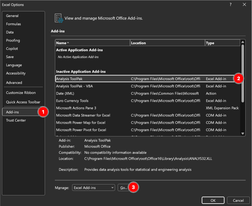 Figure 1: Excel Add-ins dialog with Analysis ToolPak enabled (Windows)
Mac users: Go to Tools → Excel Add-ins instead of File → Options.
Step-by-Step: How to Calculate One-Way ANOVA in Excel
We'll use an example dataset comparing customer satisfaction scores across three age groups.
Step 1: Organize Your Data
Arrange your data in columns, with each column representing one group. Include a header row with group labels.
Example data structure:
| Age 18-25 | Age 26-40 | Age 41+ |
|---|---|---|
| 3.8 | 4.6 | 4.0 |
| 3.0 | 4.0 | 4.8 |
| 2.2 | 4.0 | 4.6 |
| 3.2 | 3.6 | 4.2 |
| 2.8 | 5.0 | 4.0 |
| ... | ... | ... |
Table 1: Customer satisfaction scores by age group (1-5 scale)
Important:
- Each column = one group
- No empty cells within columns
- Headers in first row
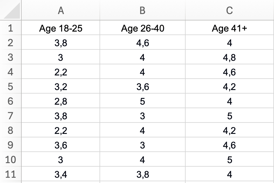 Figure 2: Proper data layout for one-way ANOVA - each age group in a separate column with descriptive headers
Step 2: Access Data Analysis
- Click the Data tab
- In the Analysis group (far right), click Data Analysis
- A dialog box will appear with analysis tools
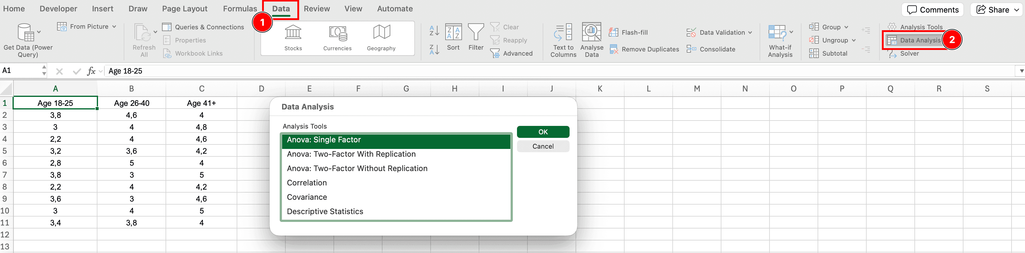 Figure 3: Data Analysis button location in Excel Data tab
Step 3: Select Anova: Single Factor
- In the Data Analysis dialog, scroll down and select Anova: Single Factor
- Click OK
"Single Factor" means one independent variable (age group). For two independent variables, you'd use "Anova: Two-Factor."
Step 4: Configure ANOVA Settings
The Anova: Single Factor dialog box appears. Configure these settings:
Input Range:
- Click the selector button and highlight all your data, including headers
- Example:
$A$1:$C$31(3 columns × 30 rows + 1 header row)
Grouped By:
- Select Columns (since each group is in a separate column)
Labels in First Row:
- Check this box if your first row contains headers
- Excel will use these labels in the output
Alpha:
- Leave as 0.05 (standard significance level)
- This is your Type I error rate threshold
Output Range:
- Select a cell where you want the results to appear (e.g.,
E1) - Or choose New Worksheet Ply for results on a new sheet
Click OK to run the analysis.
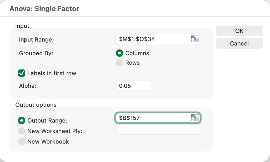 Figure 4: ANOVA Single Factor dialog configured for customer satisfaction analysis across three age groups
Step 5: Interpret ANOVA Output
Excel produces two tables: Summary and ANOVA.
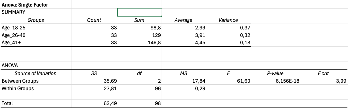 Figure 5: Complete ANOVA output showing Summary statistics and ANOVA table with significant results (F = 61.60, p < 0.001)
Summary Table
The Summary table shows descriptive statistics for each group:
- Groups: Group labels (Age 18-25, Age 26-40, Age 41+)
- Count: Sample size per group
- Sum: Total sum of values
- Average: Mean for each group
- Variance: Variance for each group
What to report: Group means (Average) and standard deviations (sqrt of Variance).
ANOVA Table
The ANOVA table shows the test results:
| Source of Variation | SS | df | MS | F | P-value | F crit |
|---|---|---|---|---|---|---|
| Between Groups | 31.44 | 2 | 15.72 | 15.43 | 0.00012 | 3.10 |
| Within Groups | 88.67 | 87 | 1.02 | — | — | — |
| Total | 120.11 | 89 | — | — | — | — |
Table 2: ANOVA output table showing significant differences between groups (p < 0.001)
Key columns explained:
SS (Sum of Squares):
- Between Groups: Variation explained by group membership
- Within Groups: Unexplained variation (error)
- Total: Between + Within
df (Degrees of Freedom):
- Between Groups: Number of groups - 1 (k - 1)
- Within Groups: Total sample size - number of groups (N - k)
MS (Mean Square):
- MS = SS / df
- Variance estimates
F (F-statistic):
- F = MS_between / MS_within
- Larger F = greater evidence of differences
P-value:
- If p < 0.05: Reject null hypothesis (groups differ significantly)
- If p ≥ 0.05: Fail to reject null hypothesis (no significant differences)
F crit (Critical F-value):
- Threshold value for significance at α = 0.05
- If F > F crit, result is significant
Example Interpretation
Hypothetical output:
- F(2, 87) = 15.43
- p-value = 0.00012 (or displayed as 1.2E-04)
- Conclusion: p < 0.05, so we reject the null hypothesis. At least one age group has significantly different satisfaction scores.
Important: ANOVA tells you that groups differ, but not which specific pairs differ. For that, you need post-hoc tests (covered later).
Testing ANOVA Assumptions
One-way ANOVA makes three assumptions. Violating these can invalidate your results.

Figure 6: ANOVA assumptions checklist - verify all three before interpreting results
Assumption 1: Independence
Requirement: Each observation must be independent. One person's score shouldn't influence another's.
How to check:
- Based on research design, not statistical test
- Ensure random sampling and no repeated measures
- Each participant appears only once in one group
Solution if violated: Use repeated measures ANOVA instead (different test).
Assumption 2: Normality
Requirement: The dependent variable should be approximately normally distributed within each group.
How to check in Excel:
Method 1: Visual inspection (Histograms)
- Create a histogram for each group
- Look for roughly bell-shaped distributions
- Identify severe skewness or outliers
Method 2: F-max test for rough check
- Calculate variance for each group (already in Summary table)
- Divide largest variance by smallest variance
- Rule of thumb: If ratio < 10, normality assumption is reasonable
Robustness: ANOVA is fairly robust to normality violations when:
- Sample sizes are equal across groups
- Each group has n > 30
- Data isn't severely skewed
Solution if violated:
- Transform data (log, square root, rank)
- Use Kruskal-Wallis test (non-parametric alternative)
Assumption 3: Homogeneity of Variance
Requirement: Variance should be similar across all groups (homoscedasticity).
How to check in Excel:
F-max test (Hartley's test):
- Find variance for each group in Summary table
- Calculate: F-max = Largest variance / Smallest variance
- Rule of thumb:
- F-max < 3: Assumption met ✓
- F-max 3-10: Borderline (proceed with caution)
- F-max > 10: Assumption violated ✗
Example:
- Group 1 variance: 0.64
- Group 2 variance: 0.49
- Group 3 variance: 0.36
- F-max = 0.64 / 0.36 = 1.78 < 3 ✓ Assumption met
Robustness: ANOVA is robust to moderate variance inequality when:
- Sample sizes are equal (balanced design)
- Ratio of largest to smallest n < 2:1
Solution if violated:
- Use Welch's ANOVA (available in R or SPSS, not native Excel)
- Transform data to stabilize variance
- Report violation and proceed cautiously if sample sizes are equal
Calculating Effect Size: Eta-Squared (η²)
The p-value tells you if differences exist, but effect size tells you how large those differences are. Always report effect size for ANOVA.
Eta-squared (η²) measures the proportion of total variance explained by group membership.
Formula
η² = SS_between / SS_total
How to Calculate in Excel
Using the ANOVA output table:
- Find Between Groups SS (Sum of Squares) in the ANOVA table
- Find Total SS in the ANOVA table
- In an empty cell, enter:
=B12/B14(adjust cell references to your table)
Example:
- Between Groups SS = 31.44
- Total SS = 63.11
- η² = 31.44 / 63.11 = 0.498 or 49.8%
Interpreting Eta-Squared
Cohen's guidelines:
- η² = 0.01: Small effect (1% of variance explained)
- η² = 0.06: Medium effect (6% of variance explained)
- η² = 0.14: Large effect (14% of variance explained)
Example interpretation: "Age group explained 49.8% of the variance in satisfaction scores, representing a very large effect size."
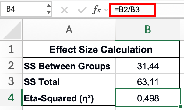 Figure 7: Calculating eta-squared effect size - divide Between Groups SS (31.44) by Total SS (63.11) to get η² = 0.498
Important: Effect size is independent of sample size and significance. You can have a statistically significant result (p < 0.05) with a small effect size (η² = 0.02) if your sample is large enough. Always interpret both.
Post-Hoc Tests: Which Groups Differ?
ANOVA only tells you that at least one group differs. To identify which specific pairs differ, run post-hoc tests.
The Multiple Comparison Problem
With 3 groups, you have 3 pairwise comparisons:
- Group 1 vs Group 2
- Group 1 vs Group 3
- Group 2 vs Group 3
Running 3 separate t-tests inflates Type I error. The solution: Bonferroni correction.
Bonferroni Correction in Excel
Bonferroni method: Divide your alpha by the number of comparisons.
Steps:
-
Calculate number of comparisons: k(k-1)/2
- For 3 groups: 3(2)/2 = 3 comparisons
- For 4 groups: 4(3)/2 = 6 comparisons
-
Calculate adjusted alpha: α_adjusted = 0.05 / number of comparisons
- For 3 groups: 0.05 / 3 = 0.017
-
Run pairwise t-tests:
- Use Data Analysis → t-Test: Two-Sample Assuming Equal Variances
- Compare each pair of groups
- Only declare significant if p < 0.017 (not 0.05)
-
Interpret:
- Groups with p < 0.017 differ significantly
- Groups with p ≥ 0.017 do not differ significantly
Example results:
- Group 1 vs Group 2: p = 0.004 < 0.017 → Significant ✓
- Group 1 vs Group 3: p = 0.001 < 0.017 → Significant ✓
- Group 2 vs Group 3: p = 0.234 > 0.017 → Not significant ✗
Conclusion: Group 1 differs from both Group 2 and Group 3, but Groups 2 and 3 don't differ from each other.
Note: Bonferroni is conservative (reduces power). For more advanced post-hoc tests (Tukey HSD, Scheffé), use SPSS, R, or the Real Statistics Excel add-in.
Reporting ANOVA Results in APA Format
Always report ANOVA results with these components:
1. Descriptive Statistics Table
Create a table showing means and standard deviations for each group:
| Age Group | n | M | SD |
|---|---|---|---|
| 18-25 | 30 | 3.2 | 0.8 |
| 26-40 | 30 | 4.1 | 0.7 |
| 41+ | 30 | 4.3 | 0.6 |
Table 3: Descriptive statistics for satisfaction scores by age group (M = mean; SD = standard deviation)
2. ANOVA Results Statement
Report the test statistic in this format:
A one-way ANOVA revealed significant differences in satisfaction scores across age groups, F(2, 87) = 15.43, p < .001, η² = 0.26.
Template:
A one-way ANOVA [revealed significant differences / revealed no significant differences] in [DV] across [IV], F([df_between], [df_within]) = [F-value], p [< .001 / = .xxx], η² = [effect size].
Formatting notes:
- Italicize F, p, and η²
- Report exact p-values if p ≥ .001 (e.g., p = .023)
- Report p < .001 for very small p-values (don't report p = .000)
- Round F to 2 decimals, p to 3 decimals, η² to 2 decimals
3. Post-Hoc Results (if ANOVA significant)
Post-hoc comparisons using the Bonferroni correction indicated that the 18-25 age group (M = 3.2, SD = 0.8) scored significantly lower than both the 26-40 age group (M = 4.1, SD = 0.7, p = .004) and the 41+ age group (M = 4.3, SD = 0.6, p = .001). The 26-40 and 41+ groups did not differ significantly from each other (p = .234).
Complete Example (Results Section)
Satisfaction Differences Across Age Groups
Descriptive statistics are presented in Table 1. A one-way ANOVA was conducted to compare satisfaction scores across three age groups (18-25, 26-40, 41+). The assumption of homogeneity of variance was met (F-max = 1.78). The ANOVA revealed significant differences in satisfaction scores across age groups, F(2, 87) = 15.43, p < .001, η² = 0.26, indicating a large effect size.
Post-hoc pairwise comparisons using the Bonferroni correction revealed that the 18-25 age group (M = 3.2, SD = 0.8) scored significantly lower than both the 26-40 age group (M = 4.1, SD = 0.7, p = .004) and the 41+ age group (M = 4.3, SD = 0.6, p = .001). The 26-40 and 41+ groups did not differ significantly from each other (p = .234). These results suggest that customer satisfaction increases with age, with younger customers (18-25) reporting lower satisfaction than older age groups.
Common ANOVA Mistakes to Avoid
1. Running multiple t-tests instead of ANOVA
- ✗ Wrong: Running t-tests for all pairs without correction
- ✓ Correct: Use ANOVA first, then post-hoc tests
2. Not checking assumptions
- ✗ Wrong: Running ANOVA blindly
- ✓ Correct: Test normality and homogeneity of variance
3. Reporting only p-values
- ✗ Wrong: "The groups differed significantly (p < .05)"
- ✓ Correct: Report F-statistic, degrees of freedom, p-value, AND effect size
4. Stopping after ANOVA is significant
- ✗ Wrong: Concluding "groups differ" without identifying which pairs
- ✓ Correct: Run post-hoc tests to identify specific differences
5. Using ANOVA for two groups
- ✗ Wrong: ANOVA with 2 groups
- ✓ Correct: Use independent samples t-test for 2 groups
Troubleshooting Common Issues
"Data Analysis button is missing"
- Solution: Enable Analysis ToolPak (see Prerequisites section)
"Input range contains non-numeric data"
- Solution: Ensure all data cells contain numbers only, no text
- Remove any empty cells within data columns
"F-statistic is very small (close to 1)"
- Interpretation: Group means are similar. No significant differences expected
- Check if you selected the correct data range
"p-value shows as scientific notation (1.2E-05)"
- Interpretation: This means p = 0.000012, which is < 0.001 (highly significant)
- Report as p < .001 in APA format
"Variances are very unequal (F-max > 10)"
- Solution 1: Transform data (log or square root transformation)
- Solution 2: Use Welch's ANOVA (requires R or SPSS)
- Solution 3: Report violation and proceed cautiously if sample sizes are equal
Next Steps: Beyond One-Way ANOVA
Note: The following advanced ANOVA techniques require statistical software like SPSS or R (Excel's Analysis ToolPak supports one-way ANOVA only).
If you have two independent variables:
- Use two-way ANOVA to test main effects and interactions
If you have repeated measures:
- Use repeated measures ANOVA (same participants tested multiple times)
If assumptions are severely violated:
- Use Kruskal-Wallis test (non-parametric alternative)
For complete survey analysis workflow:
- See our guide: How to Analyze Survey Data in Excel: Complete Guide
Frequently Asked Questions
Wrapping Up
One-way ANOVA in Excel is straightforward using the Data Analysis ToolPak:
- Organize data in columns (one per group)
- Run Anova: Single Factor via Data Analysis
- Check assumptions (independence, normality, homogeneity of variance)
- Interpret results (F-statistic and p-value)
- Calculate effect size (eta-squared)
- Run post-hoc tests (Bonferroni correction) if significant
- Report in APA format with descriptive statistics
Key takeaway: ANOVA tells you that groups differ. Post-hoc tests tell you which groups differ. Always report both the statistical significance (p-value) and practical significance (effect size).
For comparing only two groups, use our T-Test in Excel: Complete Guide. For deciding between t-test and ANOVA, see T-Test vs ANOVA: Which Test Should You Use?
References
Cohen, J. (1988). Statistical power analysis for the behavioral sciences (2nd ed.). Lawrence Erlbaum Associates.
Field, A. (2018). Discovering statistics using IBM SPSS statistics (5th ed.). SAGE Publications.
Levene, H. (1960). Robust tests for equality of variances. In I. Olkin (Ed.), Contributions to probability and statistics: Essays in honor of Harold Hotelling (pp. 278-292). Stanford University Press.
Maxwell, S. E., & Delaney, H. D. (2004). Designing experiments and analyzing data: A model comparison perspective (2nd ed.). Lawrence Erlbaum Associates.
Microsoft. (2024). Use the Analysis ToolPak to perform complex data analysis. Microsoft Support.
Tabachnick, B. G., & Fidell, L. S. (2019). Using multivariate statistics (7th ed.). Pearson.