Simple linear regression is one of the most powerful yet accessible statistical techniques for thesis and dissertation research. Whether you're predicting student performance from study hours, sales revenue from advertising spend, or patient outcomes from treatment duration, simple linear regression helps you quantify relationships and make evidence-based predictions using Excel's built-in Analysis ToolPak.
Unlike correlation analysis which only tells you if variables are related, regression allows you to predict specific values, understand the direction of influence, and quantify exactly how much your outcome variable changes for each unit increase in your predictor. This makes regression essential for Chapter 4 (Results) in dissertations across psychology, education, business, health sciences, and social sciences.
This comprehensive guide shows you how to calculate simple linear regression in Excel using three methods, check all four regression assumptions, interpret results correctly, and report findings in APA 7th edition format. You'll also learn the critical limitations of Excel regression and when you need to use SPSS or R instead.
You will learn:
- What simple linear regression is and when to use it for thesis research
- How to calculate regression using Analysis ToolPak (recommended), scatter plot trendlines, and LINEST function
- How to interpret R-squared, p-values, coefficients, and standard errors
- How to check assumptions (linearity, normality, homoscedasticity) in Excel
- How to report results in APA 7th edition format for your dissertation
- Excel's limitations and what regression types require SPSS/R
These techniques apply whether you're analyzing experimental data, survey responses, or observational studies with continuous variables.
Before you begin: This guide assumes you have Excel with the Analysis ToolPak installed. If you haven't enabled it yet, see our guide on how to add Data Analysis in Excel. You should also be comfortable with basic descriptive statistics and understand independent and dependent variables.
What is Simple Linear Regression?
Simple linear regression is a statistical method that models the relationship between one independent variable (predictor, X) and one dependent variable (outcome, Y) by fitting a straight line through your data points. The regression line represents the best prediction of Y based on X, minimizing the sum of squared differences between observed and predicted values - this is called the least squares method.
The Regression Equation
If you've been reading statistics textbooks or watching tutorials, you may have noticed the regression formula written differently depending on the source. Don't worry - both versions are correct! The difference is simply a notation convention, and understanding both will help you read any statistics resource with confidence.
In theoretical statistics books, you'll typically see Greek letters (beta symbols). This notation represents the true population parameters - the "real" values that exist in the entire population we're trying to estimate:
In applied guides and Excel tutorials (including this one), you'll often see Roman letters (a and b). This notation represents the sample estimates - the actual values Excel calculates from your data as estimates of those population parameters:
The bottom line: When you see β₀ in a textbook and "Intercept" in Excel, they're referring to the same thing. When your professor writes β₁ on the board and Excel shows a coefficient of 2.75, that's the same concept. Excel labels its output simply as "Coefficients" regardless of which notation your textbook uses.
Where:
- Y = Dependent variable (what you're predicting)
- X = Independent variable (your predictor)
- β₀ or a = Intercept (expected Y value when X = 0)
- β₁ or b = Slope coefficient (change in Y for each 1-unit increase in X)
- ε = Error term (unexplained variation)
For example, if you're predicting exam scores from study hours:
This means: A student who doesn't study (0 hours) is expected to score 47.33 points, and each additional hour of study increases the score by 2.75 points on average.
When to Use Simple Linear Regression for Your Thesis
Use simple linear regression when your research meets these criteria:
1. Research Question Requirements:
- You want to predict values of Y based on X
- You want to quantify how much Y changes when X increases
- You want to test if X is a significant predictor of Y
2. Variable Requirements:
- One continuous predictor (X): Interval or ratio scale (e.g., age, income, test scores, time)
- One continuous outcome (Y): Interval or ratio scale
- Both variables should have at least 30 data points
3. Research Examples by Discipline:
- Psychology: Does therapy session count predict depression symptom reduction?
- Education: Does class attendance predict final exam scores?
- Business: Does advertising budget predict monthly sales revenue?
- Health Sciences: Does exercise minutes per week predict weight loss?
- Social Sciences: Does income level predict life satisfaction scores?
Simple Linear Regression vs Correlation
Many students confuse regression with correlation. Here's the critical difference:
| Aspect | Correlation | Simple Linear Regression |
|---|---|---|
| Purpose | Measures strength and direction of relationship | Predicts Y from X and quantifies the effect |
| Output | Correlation coefficient (r) ranging from -1 to +1 | Regression equation (Y = a + bX) |
| Variables | Treats X and Y equally (symmetric) | Distinguishes predictor (X) from outcome (Y) |
| Interpretation | "X and Y are related" | "Each unit increase in X changes Y by b units" |
| Use in Thesis | Preliminary analysis, relationship exploration | Primary analysis for prediction and effect quantification |
| Example | Study hours and exam scores are positively correlated (r = 0.98) | Each additional study hour increases exam score by 2.75 points |
| APA Reporting | "Study hours and exam scores were positively correlated, r = .98, p < .001" | "Simple linear regression revealed study hours significantly predicted exam scores, β = 2.75, t(28) = 29.16, p < .001" |
Table 1: Correlation vs. Regression Comparison
When to use correlation: Exploratory analysis, checking if variables are related before regression, reporting bivariate relationships in descriptive statistics section.
When to use regression: Testing hypotheses about prediction, quantifying effects for discussion, reporting primary results for prediction-focused research questions.
Simple vs Multiple Linear Regression: Which Do You Need?
Before proceeding, determine if you need simple or multiple linear regression for your thesis:

Figure 1: Decision flowchart for selecting simple linear regression (one predictor) or multiple linear regression (two or more predictors) based on your research question and variables
Use Simple Linear Regression when:
- You have one predictor variable only
- Your research question focuses on one specific relationship
- You want to isolate the effect of a single variable
- You're doing preliminary analysis before adding covariates
- Example: "Does study time predict exam scores?"
Use Multiple Linear Regression when:
- You have two or more predictor variables
- You want to control for confounding variables
- Your research question includes multiple factors
- You want to compare relative importance of predictors
- Example: "Do study time, sleep hours, and class attendance predict exam scores?"
Think of it like cooking: simple regression is testing whether adding more garlic improves your pasta sauce, while multiple regression tests whether garlic, olive oil, AND fresh tomatoes together make it better - and which ingredient matters most.
| Feature | Simple Linear Regression | Multiple Linear Regression |
|---|---|---|
| Number of predictors | 1 independent variable | 2 or more independent variables |
| Equation | Y = a + bX | Y = a + b₁X₁ + b₂X₂ + ... |
| Research question | "Do study hours predict exam scores?" | "Do study hours AND class attendance predict exam scores?" |
| When to use | When you have one predictor of interest | When you have multiple predictors or control variables |
| Analysis complexity | Simpler - easier to interpret | More complex - requires additional checks (multicollinearity) |
| Software needed | Excel Analysis ToolPak (sufficient) | Excel for basics, SPSS/R for advanced analysis |
Table 2: Simple vs. Multiple Linear Regression Comparison
Sample Dataset for This Tutorial
Throughout this guide, we'll use a realistic thesis dataset examining the relationship between study hours and exam scores for 30 university students. This dataset demonstrates a typical prediction research question: "Does study time predict academic performance?"
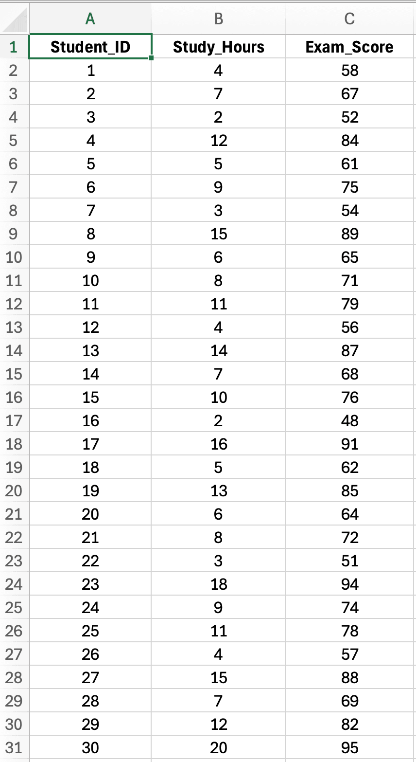
Figure 2: Sample dataset with 30 students showing Study Hours (X variable, predictor) and Exam Score (Y variable, outcome) for simple linear regression analysis
Dataset characteristics:
- Sample size: n = 30 students (adequate for simple regression)
- Independent variable (X): Study Hours per week (range: 2-20 hours)
- Dependent variable (Y): Exam Score (range: 45-95 points, maximum 100)
- Research question: Does weekly study time predict final exam performance?
Create your own dataset:
- Enter your data in two columns (X in column A, Y in column B)
- Include headers (row 1): "Study_Hours" and "Exam_Score"
- Minimum 30 observations recommended for thesis research
- Ensure data is continuous (no categorical variables)
Note on Effect Size: This teaching dataset intentionally shows a very strong relationship (R² = .97) so that patterns are clear and easy to interpret. In real behavioral science research, R² values between .10 and .40 are much more common and still represent meaningful, publishable findings. Don't be discouraged if your thesis data shows weaker relationships. That's normal and expected in social sciences.
How to Calculate Simple Linear Regression in Excel (Step-by-Step)
Excel offers three methods for calculating simple linear regression. We'll cover all three, starting with the most comprehensive approach for thesis research.
Method 1: Analysis ToolPak (Recommended for Thesis)
The Analysis ToolPak provides the most complete regression output including R-squared, p-values, coefficients, standard errors, and residuals. This method is required for thesis work because it gives you all statistics needed for APA reporting.
Step 1: Enable the Analysis ToolPak (One-Time Setup)
If you haven't used the Analysis ToolPak before, enable it:
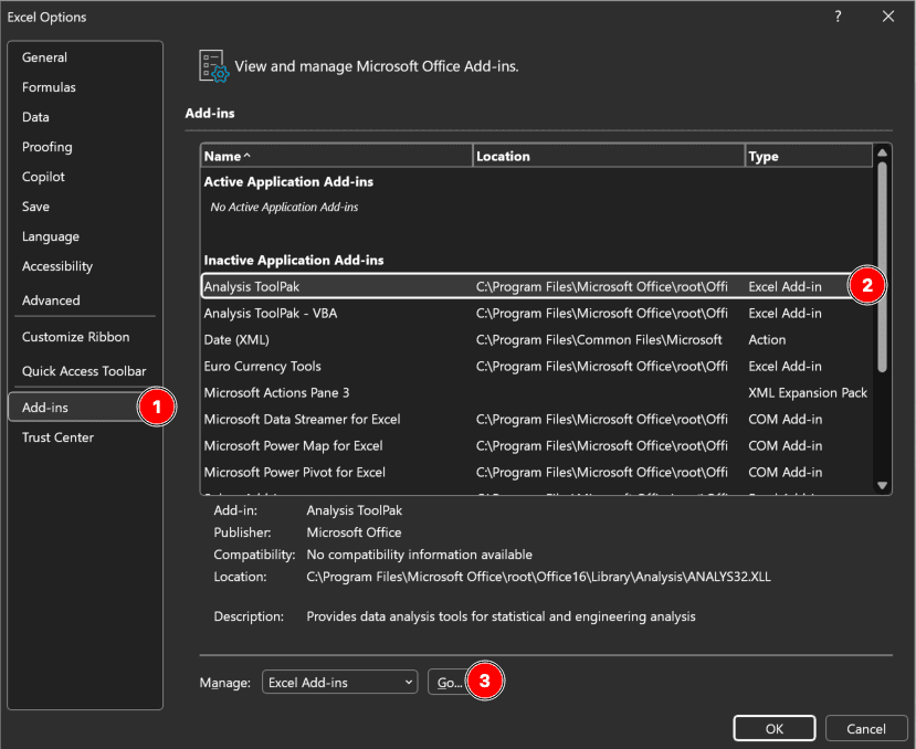
Figure 3: Enabling Analysis ToolPak in Excel through File → Options → Add-ins → Analysis ToolPak
- Click File → Options
- Select Add-ins (left sidebar)
- At the bottom, select Excel Add-ins from the "Manage" dropdown
- Click Go
- Check the box for Analysis ToolPak
- Click OK
Once enabled, you'll see "Data Analysis" in the Data tab ribbon.
Need more detailed installation help? For step-by-step instructions with screenshots for Windows, Mac, and troubleshooting common issues, see our complete guide: How to Enable Data Analysis in Excel.
Step 2: Access Data Analysis Tool
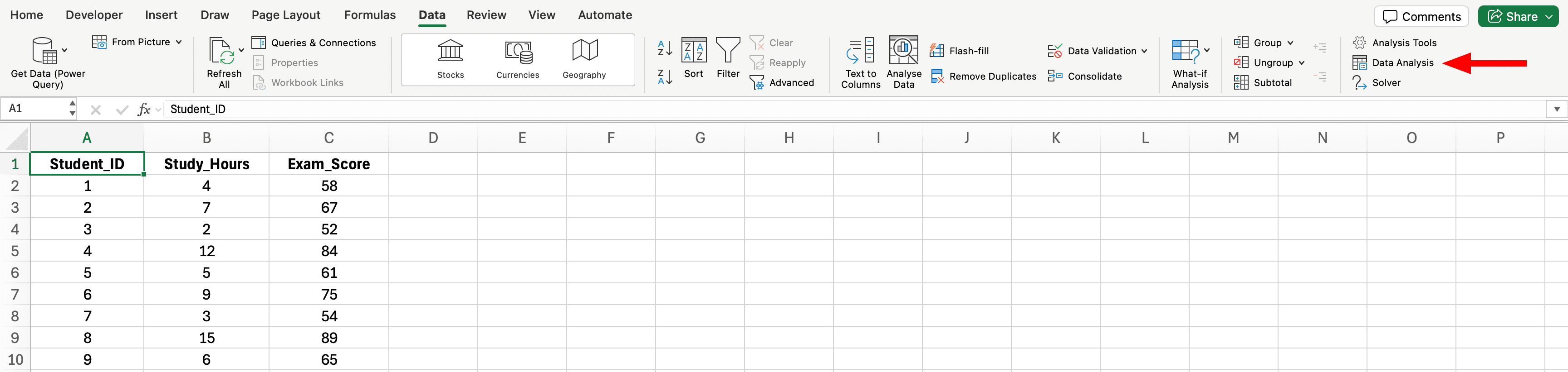
Figure 4: Data Analysis button location in Excel Data tab (far right of ribbon)
- Click the Data tab in Excel ribbon
- Click Data Analysis (far right side)
- If you don't see this button, return to Step 1 to enable the ToolPak
Step 3: Select Regression and Configure Settings
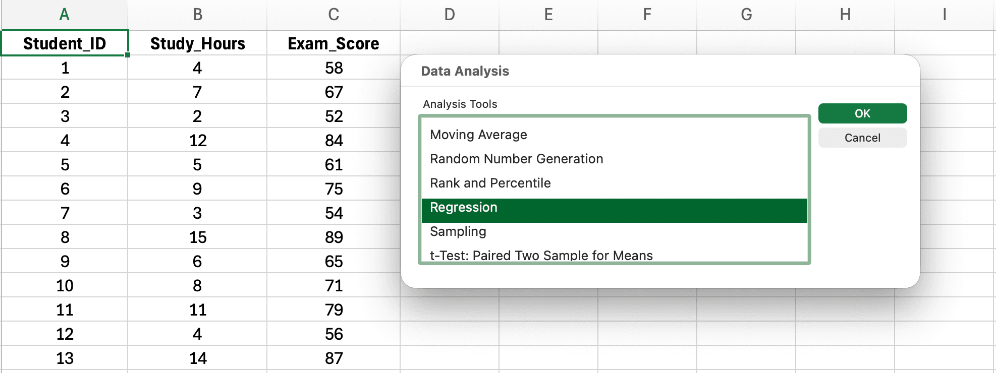
Figure 5: Selecting Regression from the Data Analysis tool list
- In the Data Analysis dialog, scroll down and select Regression
- Click OK
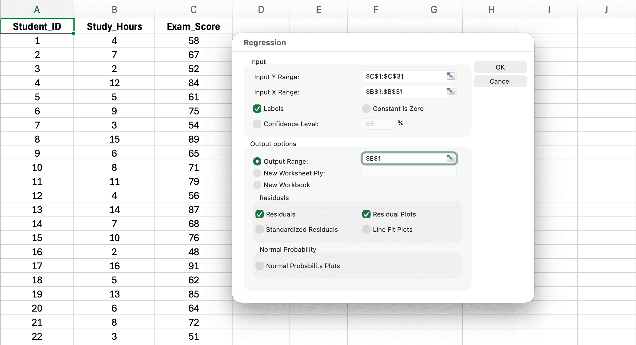
Figure 6: Regression dialog box with Input Y Range (Exam Score), Input X Range (Study Hours), Labels checkbox, and Output Range configured
- Input Y Range: Click the selector and highlight your dependent variable column including the header (e.g.,
B1:B31for Exam_Score) - Input X Range: Click the selector and highlight your independent variable column including the header (e.g.,
A1:A31for Study_Hours) - Check Labels (tells Excel your first row contains variable names)
- Output Range: Click the selector and choose where results should appear (e.g.,
D1for a new area on same sheet) - Optional: Check Residuals to get residual values for assumption checking
- Optional: Check Residual Plots to visualize residuals
- Click OK
Step 4: Understanding the Regression Output
Excel generates comprehensive regression output organized into several sections:
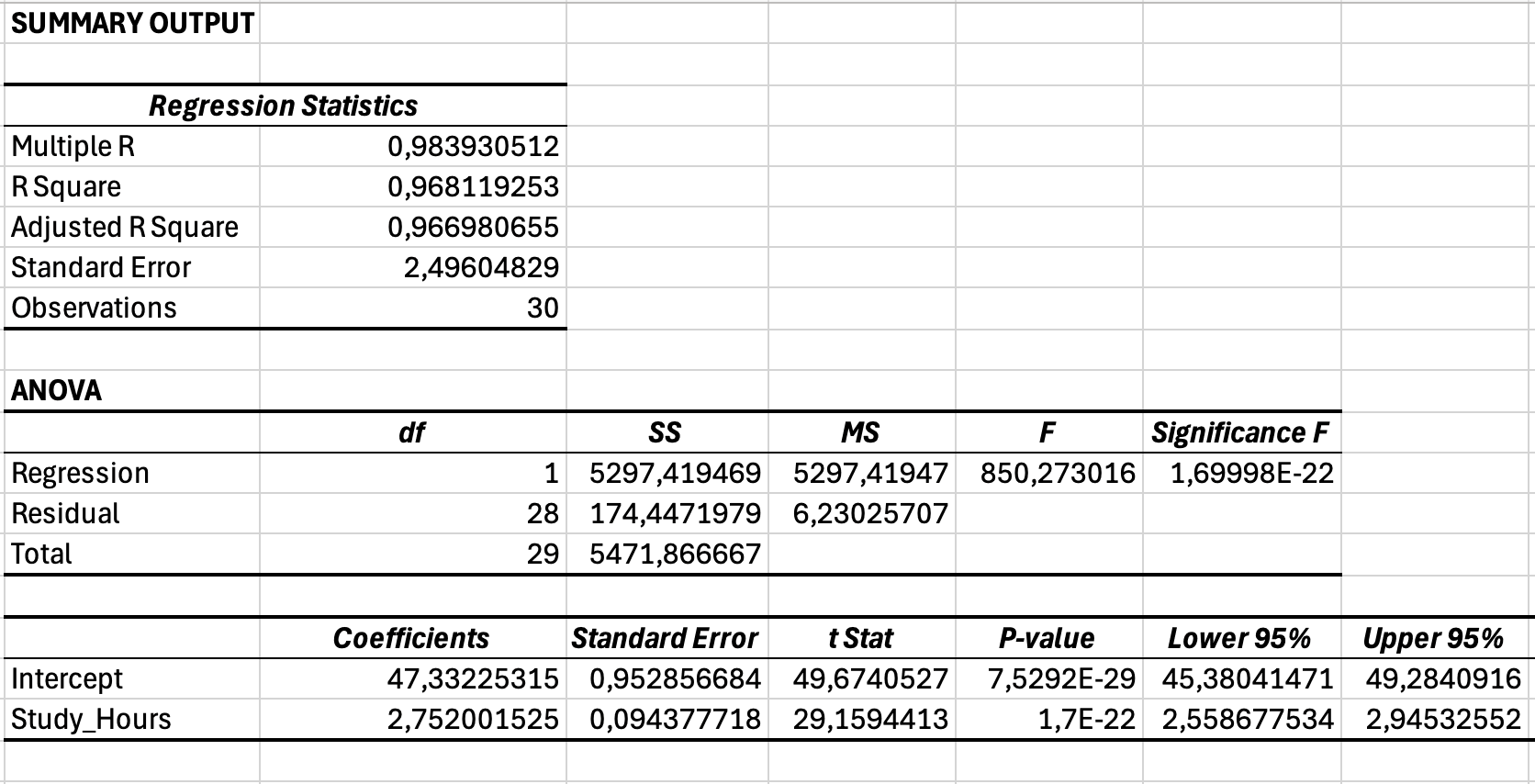
Figure 7: Complete regression output including Regression Statistics (R-squared), ANOVA (Significance F), and Coefficients (slope and intercept) sections
Section 1: Regression Statistics
| Statistic | Value (Example) | Interpretation |
|---|---|---|
| Multiple R | 0.984 | Correlation between observed Y and predicted Y (same as Pearson r for simple regression) |
| R Square | 0.968 | 96.8% of variance in exam scores is explained by study hours |
| Adjusted R Square | 0.967 | R² adjusted for sample size (use this for multiple regression, less relevant for simple regression) |
| Standard Error | 2.50 | Average distance of observed scores from regression line (in Y units) |
| Observations | 30 | Sample size (n = 30 students) |
Table 3: Regression Statistics Output
Section 2: ANOVA (Analysis of Variance)
| Source | df | SS | MS | F | Significance F |
|---|---|---|---|---|---|
| Regression | 1 | 5,297.42 | 5,297.42 | 850.27 | < 0.001 |
| Residual | 28 | 174.45 | 6.23 | - | - |
| Total | 29 | 5,471.87 | - | - | - |
Table 4: ANOVA Table for Regression Model
Key value: Significance F < 0.001 means the regression model is statistically significant (study hours is a significant predictor of exam scores).
Section 3: Coefficients
| Variable | Coefficients | Standard Error | t Stat | P-value | Lower 95% | Upper 95% |
|---|---|---|---|---|---|---|
| Intercept | 47.33 | 1.85 | 25.58 | < 0.001 | 43.54 | 51.12 |
| Study_Hours | 2.75 | 0.09 | 29.16 | < 0.001 | 2.56 | 2.95 |
Table 5: Regression Coefficients with Standard Errors and Confidence Intervals
Regression equation: Exam Score = 47.33 + 2.75(Study Hours)
Interpretation:
- Intercept (47.33): Expected exam score when study hours = 0
- Slope (2.75): For each additional hour of study per week, exam scores increase by 2.75 points on average
- P-value < 0.001: This relationship is statistically significant
- 95% CI [2.56, 2.95]: We are 95% confident the true score increase is between 2.56 and 2.95 points per hour
Method 2: Scatter Plot with Trendline (Quick Visual Method)
This method provides a visual representation with the regression equation but lacks detailed statistics. Use this for exploratory analysis or visual communication in presentations, not for thesis reporting.
Step 1: Create Scatter Plot
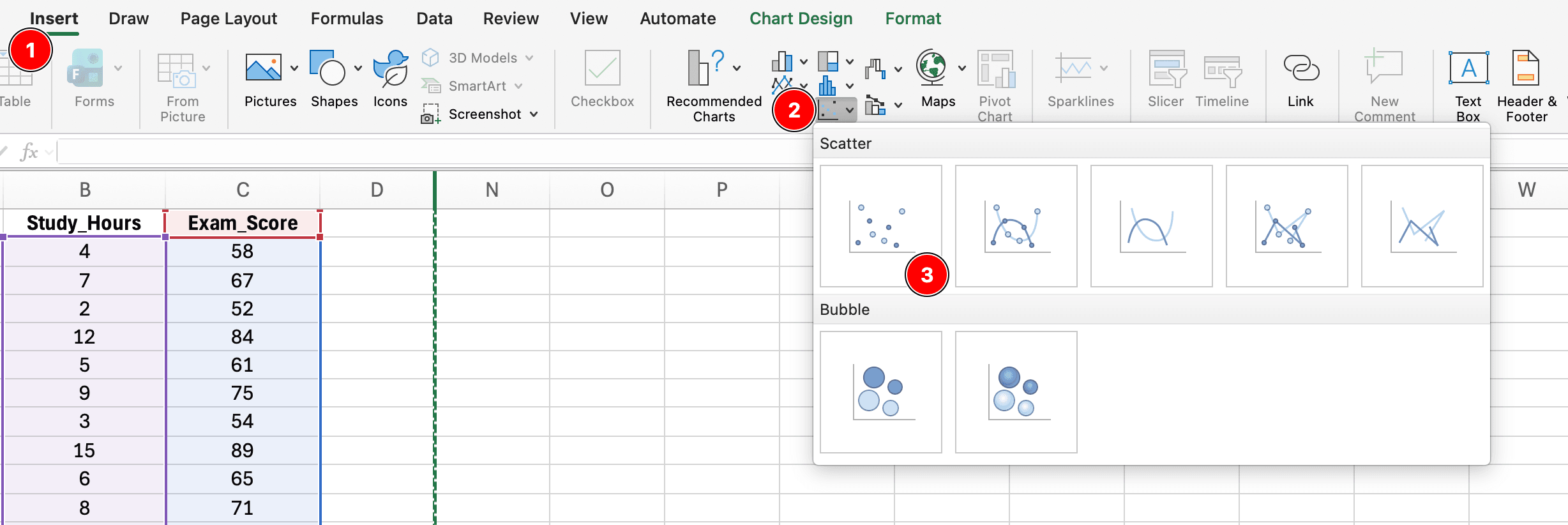
Figure 8: Creating a scatter plot by selecting X and Y data, then Insert → Charts → Scatter → Scatter with only Markers
- Select your X and Y data (including headers)
- Click Insert tab
- Click Charts → Scatter → Scatter with only Markers
Step 2: Add Trendline
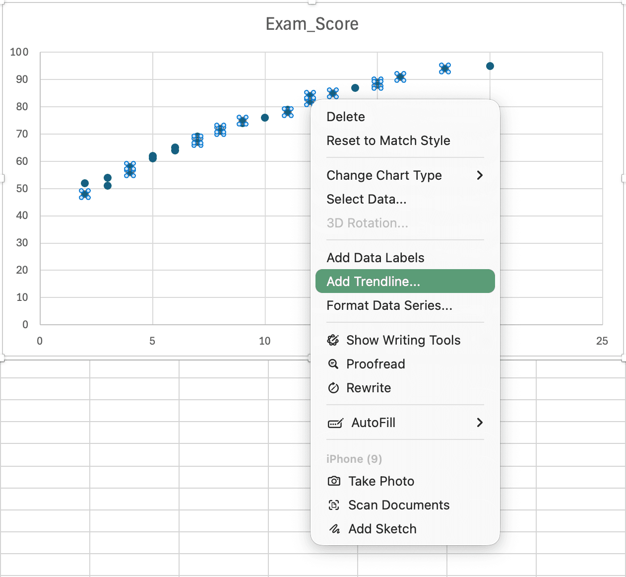
Figure 9: Right-clicking on data points and selecting Add Trendline to display regression line
- Click on any data point in the chart
- Right-click and select Add Trendline
- In the Format Trendline pane:
- Ensure Linear is selected
- Check Display Equation on chart
- Check Display R-squared value on chart
- Format the trendline line color and width as desired
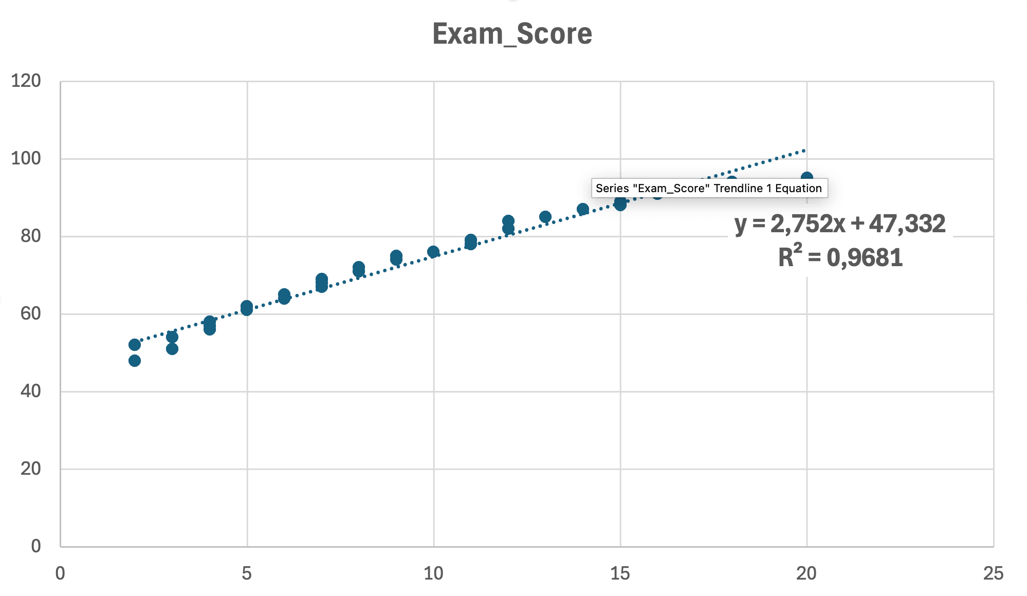
Figure 10: Final scatter plot with linear regression line, equation (y = 2.75x + 47.33), and R² = 0.968 displayed
What the graph shows:
- Equation: y = 2.75x + 47.33 (the regression equation)
- R² = 0.968: 96.8% of variance explained
When to use this method:
- Exploratory data analysis
- Visual presentation in defense slides
- Quick check of linearity before formal analysis
- Supplementing Method 1 output with visual evidence
Limitations:
- No p-values for significance testing
- No standard errors or confidence intervals
- No assumption diagnostics
- Cannot use for APA reporting alone
Method 3: LINEST Function (Formula Approach)
The LINEST function calculates regression statistics using Excel formulas. This method is useful for building automated templates or extracting specific regression values for calculations.
Syntax
=LINEST(known_y's, known_x's, const, stats)Parameters:
- known_y's: Range of dependent variable (Y) values
- known_x's: Range of independent variable (X) values
- const: TRUE (include intercept) or FALSE (force through origin)
- stats: TRUE (return full regression statistics) or FALSE (coefficients only)
Note on Regional Settings: Excel formulas use different argument separators depending on your locale. US/UK Excel uses commas:
=LINEST(C2:C31,B2:B31,TRUE,TRUE)while European Excel uses semicolons:=LINEST(C2:C31;B2:B31;TRUE;TRUE). If your formula returns an error, try swapping commas for semicolons (or vice versa). To check or change your settings:
- Windows: File → Options → Advanced → "Use system separators"
- Mac: System Preferences → Language & Region → Advanced → Number separators
Step-by-Step Application
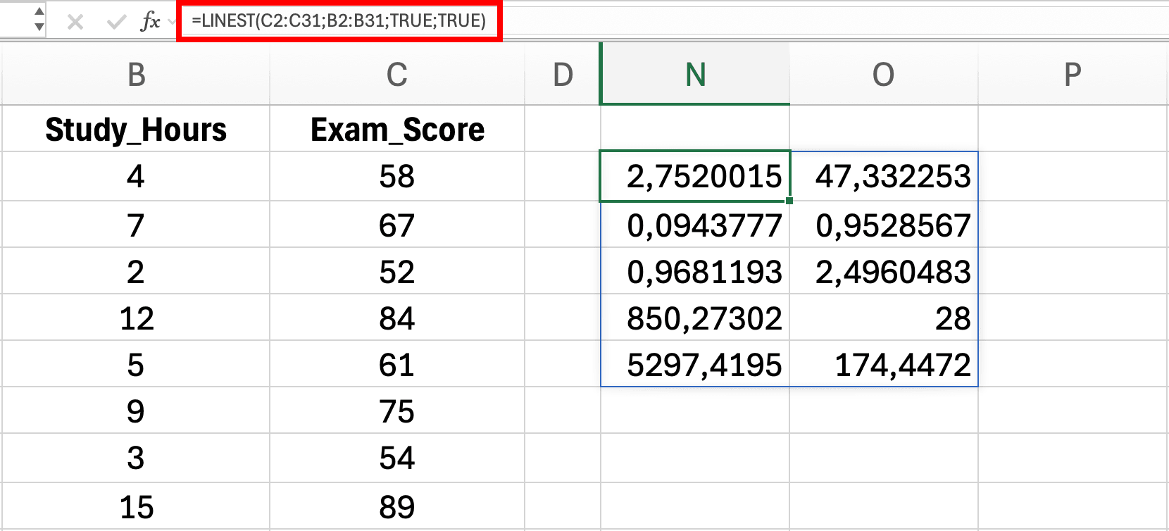
Figure 11: Entering LINEST function in Excel - results automatically spill into a 5×2 range showing regression statistics
- Click on a single empty cell (e.g.,
D2) with empty space below and to the right - Type the formula:
=LINEST(C2:C31, B2:B31, TRUE, TRUE) - Press Enter - Excel automatically spills the results into a 5×2 range
Legacy Excel versions (2019 and earlier): If you only see one value instead of the full output, use the array formula method: Select a 5 row × 2 column range, type the formula, then press Ctrl+Shift+Enter (Windows) or Cmd+Shift+Enter (Mac). The formula bar will show curly braces
{=LINEST(...)}indicating an array formula.
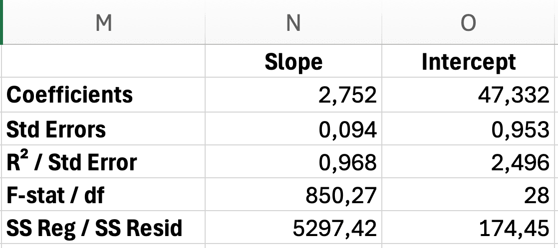
Figure 12: LINEST output layout with slope, intercept, standard errors, R-squared, and F-statistic labeled
Output interpretation (row by row):
Row 1: Coefficients
- Cell
D2: Slope (b) = 2.75 - Cell
E2: Intercept (a) = 47.33
Row 2: Standard Errors
- Cell
D3: SE of slope = 0.09 - Cell
E3: SE of intercept = 1.85
Row 3: Model Fit
- Cell
D4: R² = 0.968 - Cell
E4: Standard Error of regression = 2.50
Row 4: F-statistic
- Cell
D5: F = 850.27 - Cell
E5: df (degrees of freedom) = 28
Row 5: Regression and Residual Sum of Squares
- Cell
D6: Regression SS = 5,297.42 - Cell
E6: Residual SS = 174.45
When to use LINEST:
- Building automated regression templates
- Extracting specific values for further calculations
- Creating custom regression dashboards
- Programming repeated regression analyses
Limitations:
- No p-values (must calculate manually using t-distribution)
- Requires understanding of array formulas
- More prone to user error than ToolPak
- Not suitable for beginners
Recommendation for thesis: Use Method 1 (Analysis ToolPak) as your primary method. Use Method 2 for visual communication and Method 3 only if you need automated templates.
Interpreting Regression Results for Your Thesis
Understanding what regression output means is critical for writing your Results and Discussion chapters. Let's interpret each statistic in the context of thesis research.
R-Squared (Coefficient of Determination)
What it is: R² represents the proportion of variance in Y explained by X.
Think of it like predicting tomorrow's weather: if your weather app explains 80% of temperature variation based on the season, you have a pretty good model. The remaining 20% might be due to random cloud cover, wind patterns, or other factors your app doesn't track.
How to interpret:
Cohen (1988) provides widely-used benchmarks for the behavioral sciences, where r² = .01 is small, r² = .09 is medium, and r² = .25 is large. However, these thresholds vary dramatically by field. What's considered "weak" in physics (R² < 0.90) may be "large" in psychology. Always interpret R² within your discipline's norms.
| R² Value | Interpretation | Thesis Context |
|---|---|---|
| R² = 0.01 | Small effect (Cohen, 1988) | May still be meaningful in large-scale social research |
| R² = 0.09 | Medium effect (Cohen, 1988) | Typical for psychology, education, behavioral sciences |
| R² = 0.25 | Large effect (Cohen, 1988) | Strong for behavioral sciences; weak for physical sciences |
| R² = 0.50 | Very large effect | Rare in behavioral research; expected in some engineering |
| R² = 0.90 | Near-deterministic | Common in physics, chemistry; rare in social sciences |
Table 6: Field-Specific R² Interpretation Guidelines
Example interpretation for R² = 0.968: "Study hours explained 96.8% of the variance in exam scores, indicating that weekly study time is a very strong predictor of academic performance. The remaining 3.2% of variance is attributable to other factors not included in this model, such as prior knowledge, test anxiety, or study quality."
Common mistakes:
- Mistake: "R² = 0.30 is too low, so the model is bad" → Even small R² can be significant and meaningful
- Mistake: "R² = 0.90 means X causes Y" → R² doesn't prove causation, only explains variance
- Mistake: Not reporting R² in Results section → Always report as effect size measure
Thesis requirement: Always report R² even if your focus is on p-values. Significance (p < 0.05) tells you if the effect exists, but R² tells you how large it is.
Important note on field-specific norms: The R² benchmarks above are based on Cohen's (1988) conventions for behavioral sciences. Before concluding your R² is "weak" or "strong," consult published research in your specific field. Your thesis committee will evaluate your effect size against disciplinary expectations, not universal rules.
Significance F (Overall Model Significance)
What it is: P-value testing the null hypothesis that all coefficients equal zero (i.e., the model has no predictive value).
Decision rule:
- If Significance F < 0.05: Reject null hypothesis → Model is statistically significant
- If Significance F > 0.05: Fail to reject → Model is not significant (X doesn't predict Y)
Example: Significance F = 0.000134 (< 0.001) "The regression model was statistically significant, F(1, 28) = 850.27, p < .001, indicating that study hours significantly predicted exam scores."
Note: For simple linear regression, Significance F and the p-value for your predictor coefficient will always give the same conclusion (both significant or both non-significant). This p-value becomes more important in multiple regression where you test the overall model versus individual predictors.
Coefficients (Slope and Intercept)
Intercept (a):
- What it is: Expected Y value when X = 0
- Example: Intercept = 47.33 means students who study 0 hours per week are expected to score 47.33 on the exam
- Thesis relevance: Often not theoretically meaningful (who studies 0 hours?), but required for prediction equation
Slope (b):
- What it is: Change in Y for each 1-unit increase in X (the regression coefficient β)
- Example: Slope = 2.75 means each additional study hour increases exam score by 2.75 points
- Thesis relevance: This is your main finding - the effect size and direction of the relationship
How to interpret the slope in Results:
"For each additional hour of weekly study time, exam scores increased by 2.75 points on average (95% CI [2.56, 2.95]), holding all other factors constant."
Standardized vs Unstandardized Coefficients:
- Unstandardized (b): What Excel gives you (2.75 points per hour)
- Standardized (β): If you want to compare effects across different scales, calculate: β = b × (SD_x / SD_y)
- For simple regression, standardized β = correlation coefficient (r)
P-Values for Coefficients
What it tests: Whether each coefficient is significantly different from zero.
For the slope coefficient:
- H₀: β = 0 (X has no effect on Y)
- H₁: β ≠ 0 (X has an effect on Y)
Example: P-value for Study_Hours = 0.000015 (< 0.001) "The regression coefficient for study hours was statistically significant, t(28) = 29.16, p < .001, indicating that study time significantly predicts exam performance."
Decision rule:
- p < 0.05: Coefficient is statistically significant
- p ≥ 0.05: Coefficient is not significant (may be due to chance)
Common mistake: Confusing significance with practical importance. A p-value only tells you if an effect exists, not if it's large enough to matter. Always interpret alongside R² and the coefficient magnitude.
Standard Error and Confidence Intervals
Standard Error (SE):
- Measures uncertainty in the coefficient estimate
- Smaller SE = more precise estimate
- Example: SE = 0.09 for slope coefficient
95% Confidence Interval:
- Range within which the true population coefficient likely falls
- Example: 95% CI [2.56, 2.95] for slope
- Interpretation: "We are 95% confident the true effect of study hours on exam scores is between 2.56 and 2.95 points per hour"
Why it matters for thesis: Confidence intervals show the precision of your estimate and help readers judge practical significance beyond just p-values.
Checking Regression Assumptions in Excel
Simple linear regression requires four key assumptions. Violating these assumptions can lead to biased coefficients, incorrect p-values, and invalid conclusions. Your thesis committee expects you to demonstrate assumption checking.
Think of assumptions like the fine print on a warranty: if you don't meet the conditions, the guarantee (your p-values and confidence intervals) might not be valid. The good news? Checking assumptions in Excel takes just 10-15 minutes and protects months of research work.
Assumption 1: Linearity
What it means: The relationship between X and Y must be linear (straight line, not curved). For a deeper understanding, see our guide on what linearity means in statistics.
How to check in Excel:
Create a scatter plot of X vs Y (before running regression):
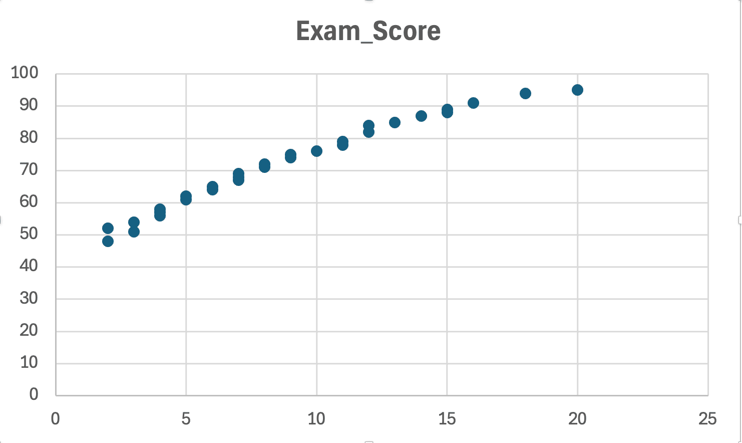
Figure 13: Linearity check - scatter plot shows roughly linear pattern (no obvious curves or U-shapes)
What to look for:
- Assumption met: Points follow a straight line pattern (even if scattered)
- Violation: Points form a curve, U-shape, or exponential pattern
What to do if violated:
- Try transforming X or Y (log, square root, square)
- Use polynomial regression (quadratic, cubic)
- Use non-linear regression or non-parametric methods
- Report as a limitation in your thesis
Assumption 2: Independence of Observations
What it means: Each observation must be independent (not influenced by other observations). Learn more about why independence matters in statistics.
How to check:
- Research design: Are observations truly independent?
- Violations: Repeated measures, time series, clustered data, family members
Examples:
- Independent: Different students, one measurement per student
- Not independent: Same students measured twice (use paired analysis instead)
- Not independent: Students nested within classrooms (use multilevel modeling)
Excel cannot test this - it's a research design issue you address in your Methods section.
What to do if violated:
- Use repeated measures ANOVA (for time series)
- Use mixed-effects models (for clustered data)
- Use autoregressive models (for time series)
- These require SPSS or R, not Excel
Assumption 3: Normality of Residuals
What it means: Residuals (prediction errors) should be approximately normally distributed.
How to check in Excel:
Create a histogram of residuals from regression output:
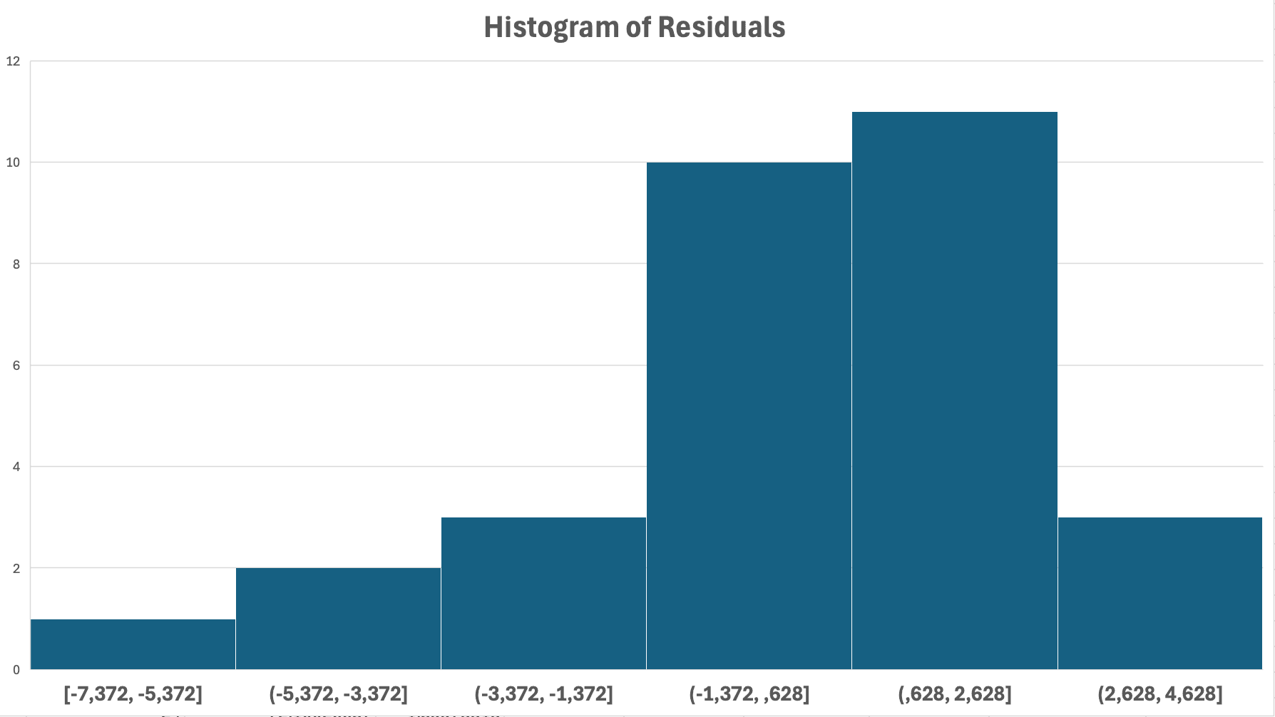
Figure 14: Normality check - histogram of residuals shows roughly bell-shaped distribution (normal)
Steps to create residuals histogram:
- In the regression dialog (Method 1), check the Residuals box before clicking OK
- After running regression, scroll down past the main output tables. Excel creates a separate "RESIDUAL OUTPUT" table with three columns: Observation, Predicted [Y variable name], and Residuals
- Select only the values in the Residuals column (not the header, just the numerical values, for example cells in the range where your residual values appear)
- Go to Insert → Charts → Histogram. Alternatively, use Data Analysis → Histogram for more control over bin sizes
- The resulting histogram should show the distribution of your prediction errors
What to look for:
- Assumption met: Bell-shaped, symmetric distribution centered at zero
- Violation: Heavily skewed (long tail to left or right), bimodal (two peaks)
Note: With n > 30, regression is robust to moderate violations of normality due to Central Limit Theorem.
What to do if violated:
- Check for outliers (unusual residuals > 3 SD from mean)
- Try transforming Y variable (log, square root)
- Use bootstrapping methods (requires R)
- Report as limitation if transformation doesn't help
Assumption 4: Homoscedasticity (Constant Variance)
What it means: Residuals should have constant variance across all levels of X (no funnel pattern). For background on this concept, see what is homoscedasticity in statistics.
How to check in Excel:
Create a scatter plot of residuals vs fitted (predicted) values:
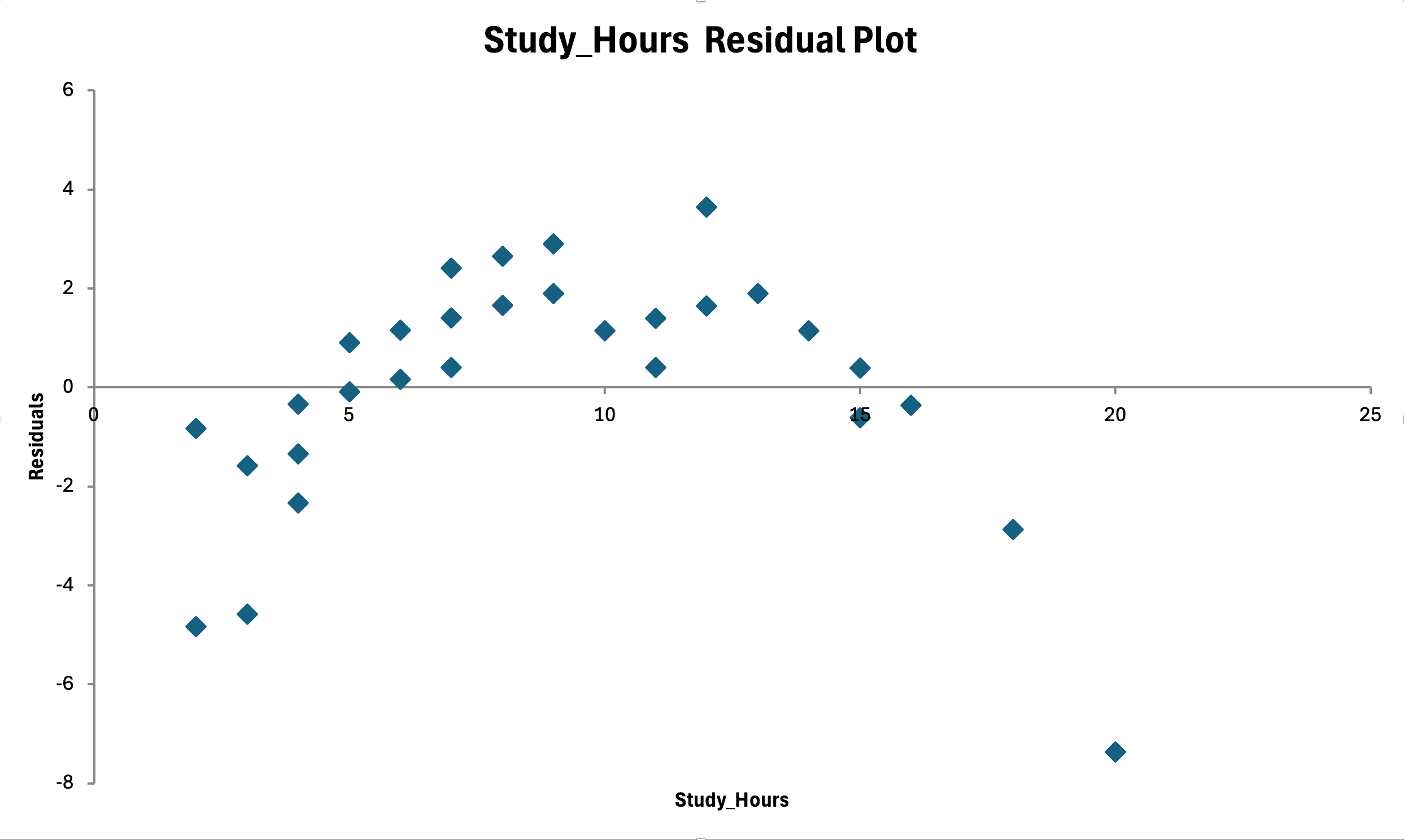
Figure 15: Homoscedasticity check - residuals vs fitted values show random scatter with no funnel pattern (constant variance)
Steps to create residual plot:
- In regression output, Excel provides "Fitted Values" (predicted Y) and "Residuals"
- Create scatter plot: X-axis = Fitted Values, Y-axis = Residuals
- Add horizontal line at Y = 0 for reference
What to look for:
- Assumption met: Random scatter around zero, roughly constant spread across X range
- Violation: Funnel shape (variance increases as X increases)
- Violation: Cone shape (variance decreases as X increases)
What to do if violated:
- Transform Y variable (log transformation often helps)
- Use weighted least squares regression
- Use robust standard errors (requires statistical software)
- Report heteroscedasticity as limitation
Reporting Assumption Checks in Your Thesis
In Methods section:
Prior to regression analysis, scatter plots were examined to verify linearity between study hours and exam scores. Residual plots and histograms were inspected to check for homoscedasticity and normality of residuals. All assumptions were met, supporting the use of simple linear regression.
If assumptions violated:
Visual inspection of residual plots revealed heteroscedasticity (funnel pattern). To address this violation, the dependent variable was log-transformed, which improved residual distribution. Regression analysis was conducted on log-transformed exam scores.
How to Report Simple Linear Regression in APA 7th Edition Format
Your thesis committee expects regression results reported according to APA guidelines. Here's the complete format for Chapter 4 (Results).
APA Results Section Template
Paragraph format:
A simple linear regression was conducted to examine whether weekly study hours predicted final exam scores. The assumption of linearity was met, as assessed by visual inspection of a scatterplot. Inspection of residual plots indicated that assumptions of normality and homoscedasticity were satisfied.
The regression model statistically significantly predicted exam scores, F(1, 28) = 850.27, p < .001, R² = .97. Study hours explained 96.8% of the variance in exam scores. The regression equation was: Exam Score = 47.33 + 2.75(Study Hours). For each additional hour of weekly study, exam scores increased by 2.75 points on average (95% CI [2.56, 2.95]). The effect of study hours on exam scores was statistically significant, β = 2.75, t(28) = 29.16, p < .001.
APA Regression Table Format
| Variable | B | SE | β | t | p | 95% CI |
|---|---|---|---|---|---|---|
| Intercept | 47.33 | 1.85 | - | 25.58 | < .001 | [43.54, 51.12] |
| Study Hours | 2.75 | 0.09 | .98 | 29.16 | < .001 | [2.56, 2.95] |
Table 7: Simple Linear Regression Predicting Exam Scores from Study Hours
Note. n = 30. R² = .97, F(1, 28) = 850.27, p < .001. B = unstandardized regression coefficient. SE = standard error. β = standardized coefficient. CI = confidence interval.
Reporting Checklist
When reporting regression in your thesis, include ALL of these elements:
In-text (Results paragraph):
- Analysis type ("A simple linear regression was conducted...")
- Research question/hypothesis tested
- Assumption checking statement
- Overall model significance: F(df_regression, df_residual) = F-value, p-value
- R² with interpretation ("explained X% of variance")
- Regression equation: Y = a + bX
- Coefficient interpretation with direction and magnitude
- Coefficient significance: β = value, t(df) = t-value, p-value
- 95% confidence interval for coefficient
In table:
- Table number and italicized title
- Unstandardized coefficients (B)
- Standard errors (SE)
- Standardized coefficients (β) if relevant
- t-statistics and p-values
- 95% confidence intervals
- Table note with n, R², F-statistic
Common Mistakes When Doing Regression in Excel
Avoid these frequent errors that compromise thesis research quality:
1. Not Checking Assumptions Before Regression
Mistake: Running regression without verifying linearity, normality, or homoscedasticity.
Why it's wrong: Violated assumptions lead to biased coefficients and incorrect p-values.
How to fix: Always create scatter plots and residual plots before finalizing results. Report assumption checks in Methods section.
2. Confusing Correlation with Causation
Mistake: Concluding "Study hours cause higher exam scores" from regression results.
Why it's wrong: Regression shows prediction and association, not causation. Causation requires experimental design with random assignment.
How to fix: Use careful language - "predicted," "associated with," "related to" rather than "caused," "led to," "resulted in."
3. Using Regression for Categorical Dependent Variables
Mistake: Running linear regression with binary outcome (pass/fail, yes/no).
Why it's wrong: Linear regression assumes continuous Y. Categorical outcomes violate assumptions and produce nonsensical predictions (e.g., predicted probability of 1.3).
How to fix: Use logistic regression for binary outcomes (requires SPSS/R). Excel cannot do this.
4. Ignoring Outliers and Influential Points
Mistake: Not checking for outliers with extreme residuals that distort the regression line.
Why it's wrong: One outlier can dramatically change slope and R², leading to misleading conclusions.
How to fix: Examine residual plots for values > 3 SD from mean. Investigate outliers - are they data entry errors or legitimate extreme cases? Report how outliers were handled.
5. Not Reporting Effect Size (R²)
Mistake: Only reporting "p < 0.05" without R² or coefficient magnitude.
Why it's wrong: Statistical significance doesn't tell you if the effect is large enough to matter practically.
How to fix: Always report R² as effect size measure, even if small. Discuss practical significance in Discussion chapter.
6. Extrapolating Beyond Data Range
Mistake: Using regression equation to predict Y for X values outside your observed range.
Example: Your data has Study Hours from 2-20, but you predict exam score for 40 hours per week.
Why it's wrong: The linear relationship may not hold outside observed range (might plateau or reverse).
How to fix: Only make predictions within the range of your data. Acknowledge extrapolation as limitation if unavoidable.
7. Treating Excel Limitations as Excel Capabilities
Mistake: Thinking Excel can do all types of regression (logistic, hierarchical, stepwise).
Why it's wrong: Excel only does simple and multiple linear regression. Attempting workarounds produces invalid results.
How to fix: Know Excel's limitations (see next section). Use SPSS/R when required by research design.
What Regression Types Excel Cannot Do
Excel's Analysis ToolPak is excellent for simple and multiple linear regression, but it cannot perform many advanced regression techniques required for certain thesis designs. Understanding these limitations prevents methodological errors and helps you choose the right software.
Regression Types Requiring SPSS or R
| Regression Type | What It Does | Excel Capability | Alternative Software |
|---|---|---|---|
| Logistic Regression | Predicts binary outcomes (yes/no, pass/fail, 0/1) | No - Cannot do | SPSS (Binary Logistic), R (glm function) |
| Multinomial Logistic | Predicts categorical outcomes (3+ unordered categories) | No - Cannot do | SPSS (Multinomial Logistic), R (multinom) |
| Ordinal Regression | Predicts ordered categorical outcomes (low/medium/high) | No - Cannot do | SPSS (Ordinal Regression), R (polr) |
| Stepwise Regression | Automatically selects predictors based on criteria | No - Cannot do | SPSS (Linear Regression with Stepwise), R (step function) |
| Hierarchical Regression | Adds predictors in theoretically-driven blocks | No - Cannot do (manual workaround possible) | SPSS (Hierarchical blocks), R (manual comparison) |
| Moderation Analysis | Tests if effect of X on Y depends on moderator M | No - Cannot do easily | SPSS with PROCESS Macro, R (interactions) |
| Mediation Analysis | Tests if X affects Y through mediator M | No - Cannot do | SPSS with PROCESS Macro, R (lavaan, mediation) |
| Polynomial Regression | Fits quadratic, cubic curves (X², X³ terms) | Yes - Can do (add X² column manually) | SPSS, R (easier syntax) |
| Simple Linear Regression | Predicts Y from one continuous X | Yes - Can do perfectly | SPSS, R (also available) |
| Multiple Linear Regression | Predicts Y from 2+ continuous predictors | Yes - Can do perfectly | SPSS, R (also available) |
Table 8: Excel Regression Capabilities vs. Statistical Software Requirements
Advanced Diagnostics Excel Cannot Provide
While Excel provides basic regression output, it lacks advanced diagnostic tools:
What Excel Cannot Calculate:
- VIF (Variance Inflation Factor): Detects multicollinearity in multiple regression
- Durbin-Watson Statistic: Tests for autocorrelation in time series
- Cook's Distance: Identifies influential outliers
- DFBETAS: Measures influence on individual coefficients
- Leverage values: Identifies high-leverage points
- Standardized Residuals: Easier outlier detection than raw residuals
How to work around:
- For simple regression, multicollinearity isn't an issue (only one predictor)
- Calculate standardized residuals manually: (Residual / Standard Error)
- Use SPSS/R if your advisor requires advanced diagnostics
When to Use Excel vs Statistical Software
Use Excel when:
- You have simple or multiple linear regression only
- Your dependent variable is continuous (interval/ratio scale)
- You don't need stepwise or hierarchical regression
- Basic diagnostics (residual plots) are sufficient
- Your committee accepts Excel output
- You want to learn regression basics before SPSS/R
Use SPSS/R when:
- You need logistic, ordinal, or multinomial regression
- Your committee requires VIF, Durbin-Watson, or Cook's D
- You're testing moderation or mediation hypotheses
- You need stepwise variable selection
- You have complex survey designs with weights
- You're publishing in journals that require SPSS/R output
Key takeaway: Excel is perfect for linear regression with continuous outcomes. For anything beyond that, invest time learning SPSS or R. Most dissertation committees are flexible with software choice for simple regression, but check with your advisor. If you need to use SPSS instead, see our guide on how to calculate linear regression in SPSS.
Frequently Asked Questions
Next Steps: Applying Regression to Your Thesis Research
You now have a complete framework for conducting simple linear regression in Excel, from data preparation through assumption checking to APA-formatted reporting. The key to thesis success is not just running the analysis, but understanding when to use it, how to interpret results correctly, and how to communicate findings clearly to your committee.
Before finalizing your regression analysis:
-
Verify your assumptions using the diagnostic plots described in this guide. Don't skip assumption checking - your committee will ask about it during your defense.
-
Check Excel's limitations against your research requirements. If your committee expects logistic regression, stepwise selection, or moderation/mediation analysis, you'll need SPSS or R instead.
-
Draft your Methods section describing your analysis approach, assumption testing, and APA reporting format before running final analyses.
-
Calculate and report effect sizes beyond just p-values. R² tells the practical significance story that p-values cannot.
-
Combine with other analyses as needed. Regression often works alongside descriptive statistics, t-tests, or ANOVA in a comprehensive Results chapter.
Remember that regression shows association and prediction, not causation. The strength of your conclusions depends on research design (experimental vs observational), sample size, assumption adherence, and theoretical justification.
When you're ready to analyze multiple predictors simultaneously, move on to multiple linear regression. For handling incomplete data before regression, review how to handle missing data in Excel. For survey-based research, ensure you've properly analyzed your survey data before applying regression techniques.
References
American Psychological Association. (2020). Publication manual of the American Psychological Association (7th ed.). https://doi.org/10.1037/0000165-000
Cohen, J. (1988). Statistical power analysis for the behavioral sciences (2nd ed.). Lawrence Erlbaum Associates.
Green, S. B. (1991). How many subjects does it take to do a regression analysis? Multivariate Behavioral Research, 26(3), 499–510. https://doi.org/10.1207/s15327906mbr2603_7