How to Handle Missing Data in Excel Survey Analysis (Thesis Guide)

Missing data is one of the most common and frustrating problems you'll face when analyzing survey data in Excel for your thesis or dissertation. Whether respondents skip questions, drop out mid-survey, or provide incomplete answers, missing data threatens the validity of your research findings.

Your thesis committee will scrutinize how you handled missing data. Simply deleting rows or ignoring blank cells can introduce bias and undermine months of research work. The wrong approach can turn statistically significant results into meaningless noise, or worse, lead to false conclusions that fail to replicate.

This guide shows you exactly how to handle missing data in Excel survey analysis using methods your thesis committee will accept. You'll learn when to use listwise deletion versus mean imputation, how to diagnose missing data patterns, and most importantly, how to report your decisions in APA format for your Methods section.

By the end, you'll have a decision framework for choosing the right missing data method for your specific thesis scenario, complete with Excel formulas and APA reporting templates.

Why Missing Data Matters for Your Thesis

Missing data isn't just a technical inconvenience. It directly threatens three critical aspects of your thesis research:

Statistical Power: Every missing response reduces your sample size. If you collected 300 survey responses but 30% have missing data, you might be left with only 210 complete cases after listwise deletion. This reduced sample can drop your statistical power below acceptable levels (typically 0.80), increasing the risk of Type II errors where you fail to detect real effects.

Bias in Results: Missing data is rarely random. If younger respondents systematically skip income questions, or dissatisfied customers drop out of satisfaction surveys, your results no longer represent your target population. This bias can reverse the direction of relationships, inflate or deflate effect sizes, and lead to conclusions that don't generalize beyond your biased sample.

Validity of Conclusions: Your thesis committee knows that how you handle missing data affects the validity of every statistical test you run. Correlations, t-tests, ANOVA, and regression analyses all produce different results depending on your missing data approach. If you handle it incorrectly, your entire findings section becomes questionable.

Consider this real example: A student analyzed employee satisfaction surveys with 15% missing data on salary questions. They used mean imputation without checking patterns. Their analysis showed no relationship between salary and satisfaction. Later review revealed that low-paid employees systematically skipped salary questions because they were embarrassed. The missing data was hiding the exact relationship the thesis aimed to study.

Your thesis committee expects you to demonstrate awareness of these issues and justify your missing data decisions with methodological rigor, not convenience.

Understanding Missing Data Types

Before choosing a method to handle missing data in Excel, you need to understand what type of missing data you have. This diagnosis determines which techniques are appropriate and which will introduce bias into your thesis results.

Missing Completely at Random (MCAR)

Data is MCAR when the probability of being missing is the same for all observations, with no systematic pattern. This is the "best case" scenario for missing data.

Example: Your online survey system randomly crashed for 5% of respondents, cutting them off mid-survey regardless of their answers or demographics. Or respondents accidentally skipped questions by clicking "Next" too quickly, with no pattern to which questions or which respondents.

Key characteristic: The missing data is unrelated to any variable in your dataset, whether measured or unmeasured. If you could magically know the missing values, they would look like a random sample of the complete data.

Why it matters: MCAR is the only type where listwise deletion (simply removing incomplete cases) produces unbiased estimates. You lose statistical power from reduced sample size, but your results remain valid.

Missing at Random (MAR)

Data is MAR when the probability of being missing depends on observed variables in your dataset, but not on the missing values themselves.

Example: Older respondents systematically skip technology-related questions because they're less familiar with the terms, but among same-age respondents, the missingness is random. Or survey dropout rates differ by gender (women more likely to complete long surveys than men), but within each gender, dropout is random.

Key characteristic: You can predict which responses are likely to be missing based on other variables you measured. The missingness relates to what you observed, not to the hidden missing values.

Why it matters: MAR data requires more sophisticated handling than MCAR. Simple deletion can introduce bias because you're not equally likely to delete all types of respondents. Mean imputation becomes more acceptable if you account for the relationships between variables.

Not Missing at Random (NMAR)

Data is NMAR when the probability of being missing depends on the missing values themselves, even after accounting for other variables.

Example: Low-income respondents skip salary questions because they earn less (the missingness directly relates to the missing value). Or dissatisfied customers abandon satisfaction surveys before completion (those who would rate lowest don't provide ratings).

Key characteristic: The reason for missingness is related to what the answer would have been. You can't predict missingness from observed variables alone because the mechanism involves the unobserved data.

Why it matters: NMAR is the most problematic type for thesis research. No simple method in Excel can handle it without bias. You need advanced techniques like pattern-mixture models or sensitivity analyses, often requiring statistical software beyond Excel. For thesis purposes, high levels of NMAR data may require re-collection or major limitations acknowledgment.

How to Diagnose Your Missing Data Pattern in Excel

You cannot definitively prove data is MCAR versus MAR versus NMAR, but you can look for evidence of patterns that suggest systematic missingness.

Step 1: Calculate the percentage of missing data

Count total missing cells across your critical variables. If you have 300 respondents and 50 have missing values on at least one key variable, that's 16.7% missing data.

Step 2: Create missing data indicators

Add a new column for each variable with missing data. Code 1 for missing, 0 for present. This transforms missingness into a variable you can analyze.

Step 3: Test for relationships with observed variables

Run correlations between your missing data indicators and demographic variables (age, gender) or other survey responses. If certain groups have significantly higher missing rates, your data is not MCAR.

Step 4: Compare respondents with and without missing data

Use t-tests to compare means of observed variables between complete cases and cases with missing data. If complete cases differ systematically from incomplete cases on key variables, you have evidence against MCAR.

For thesis purposes, if you find no significant patterns, you can tentatively treat data as MCAR and justify listwise deletion. If you find patterns related to observed variables, you have MAR data. If you suspect patterns related to unobserved factors, you have NMAR and need to consult your advisor about advanced approaches or limitations.

Note on Regional Settings: Excel formulas use different argument separators depending on your locale. US/UK Excel uses commas: =IF(ISBLANK(A1),0,A1) while European Excel uses semicolons: =IF(ISBLANK(A1);0;A1). If a formula returns an error, try swapping commas for semicolons (or vice versa). To check or change your settings:

• Windows: File → Options → Advanced → Editing options → "Use system separators"
• Mac: System Preferences → Language & Region → Advanced → Number separators

Method 1: Listwise Deletion (Complete Case Analysis)

Listwise deletion, also called complete case analysis, is the simplest approach to handling missing data in Excel: delete any row that has at least one missing value on the variables you're analyzing.

When to Use Listwise Deletion

Use listwise deletion when all three conditions are met:

1. Less than 5% missing data: Your missing data percentage is small enough that losing those cases won't substantially reduce statistical power.

2. Data is MCAR: You've tested for patterns and found no evidence that missingness relates to any observed or unobserved variables.

3. Adequate sample size remains: After deletion, you still have sufficient cases for your planned analyses (typically n ≥ 30 per group for t-tests, n ≥ 15 per cell for ANOVA, n ≥ 10 per predictor for regression).

Do NOT use listwise deletion if:

• You have more than 10% missing data (too much power loss)
• Missing data shows systematic patterns (introduces bias)
• Your remaining sample size falls below minimum requirements
• Different analyses would use different subsets of cases (makes results non-comparable)

Step-by-Step: Listwise Deletion in Excel

Step 1: Identify rows with missing data

First, you need to find which rows have any missing values in your key analysis variables.

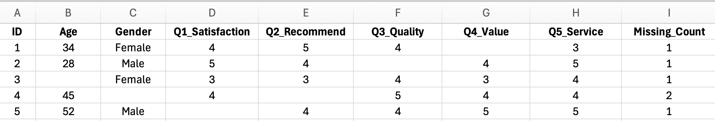
Figure 1: Survey dataset with missing data in Excel - blank cells indicating missing responses

Add a helper column (e.g., column Z) with this formula in row 2:

=COUNTBLANK(B2:Y2)

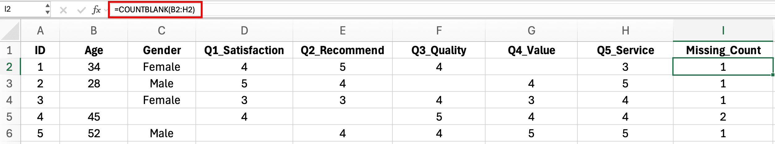
Figure 2: Excel COUNTBLANK formula to identify rows with missing data - helper column showing count of blank cells

This counts blank cells in your data range for that row. Drag the formula down for all respondents. Any row with a value greater than 0 has missing data.

Step 2: Filter to complete cases only

Apply AutoFilter to your dataset (Data > Filter). Click the dropdown in your helper column and uncheck any value except 0. This shows only complete cases.

Alternatively, use this formula to create a filtered dataset on a new sheet:

=FILTER(A2:Y1000, Z2:Z1000=0, "No complete cases")

Figure 3: Excel FILTER formula creating a dataset with only complete cases - no missing data

This copies only rows where the helper column equals 0 (complete data).

Step 3: Verify your remaining sample size

Count your complete cases and calculate the percentage deleted. If you started with 300 respondents and have 285 complete cases, you deleted 15 (5%). Document this for your Methods section.

Step 4: Perform your analyses on complete cases

Run all your statistical tests (Cronbach's Alpha, descriptive statistics, t-tests, ANOVA, correlation) on this filtered dataset of complete cases only.

Advantages and Limitations for Thesis Research

Advantages:

• Simple to implement in Excel with basic formulas
• Produces unbiased estimates if data is truly MCAR
• Easy to explain and defend to thesis committee
• Standard approach in most published research
• No assumptions about the shape of distributions

Limitations:

• Reduces statistical power by shrinking sample size
• Wasteful if you have different missing patterns across analyses
• Can introduce bias if MCAR assumption is violated
• Different analyses might use different subsets, making comparisons difficult
• May drop cases you spent time and money collecting

How to Report Listwise Deletion in APA Format

Your Methods section should include a missing data subsection that reports:

Missing data analysis revealed that 47 of 312 respondents (15.1%) had at least one missing value across the variables of interest. Comparison of respondents with complete versus incomplete data showed no significant differences in age, t(310) equals 1.23, p equals .22, gender distribution, χ²(1) equals 0.87, p equals .35, or baseline satisfaction scores, t(310) equals 0.65, p equals .52, suggesting data were missing completely at random. Listwise deletion was applied, resulting in a final analytic sample of n equals 265 for all subsequent analyses.

Key elements to include:

• Number and percentage of cases with missing data
• Statistical tests showing no systematic differences (supporting MCAR)
• Final sample size after deletion
• Statement that all analyses use the same complete-case dataset

Method 2: Mean/Median Imputation

Mean imputation replaces missing values with the mean (or median) of the observed values for that variable. This is one of the most common methods students use in Excel because it's intuitive and preserves sample size.

When to Use Mean/Median Imputation

Use mean or median imputation when:

1. Numeric scale variables: You're imputing Likert scale responses, continuous measurements, or count data (not categorical variables).

2. 5-10% missing data: You have enough missingness that deletion would hurt power, but not so much that imputation distorts distributions.

3. MAR or MCAR patterns: Missing data is random or related only to observed variables you're not currently analyzing.

4. Single-variable missingness: Respondents have missing data on one variable but complete data on others.

Use median instead of mean when:

• Your data has outliers that skew the mean
• Your variable is ordinal (Likert scales 1-5, 1-7)
• You want a more conservative imputation
• Your distribution is non-normal

Do NOT use mean/median imputation if:

• You're imputing categorical variables (use mode or category creation instead)
• Missing data is NMAR (depends on the missing values themselves)
• You'll calculate correlations or regression (imputation reduces correlations artificially)
• You need to preserve variance for advanced analyses

Step-by-Step: Mean Imputation in Excel

Let's say you have a satisfaction scale (1-7) in column C with some missing responses.

Step 1: Calculate the mean of observed values

In a helper cell (e.g., C1), calculate the mean excluding blanks:

=AVERAGE(C2:C1000)

If your data has text or errors, use:

=AVERAGEIF(C2:C1000, ">0")

This gives you the mean to impute. Let's say it's 4.8.

Step 2: Create imputed variable with formula

In a new column (e.g., D2), use this formula:

=IF(ISBLANK(C2), $C$1, C2)

This says: "If C2 is blank, use the mean from C1, otherwise use the original value from C2." The dollar signs lock the reference to your mean cell.

Drag this formula down for all respondents. You now have a complete variable with missing values replaced by the mean.

Figure 4: IF ISBLANK formula in Excel replacing missing values with mean for imputation

Step 3: Verify the imputation

Count how many values were imputed:

=COUNTIF(C2:C1000, "")

Compare the mean of your imputed variable to your original:

Original mean: =AVERAGE(C2:C1000)
Imputed mean: =AVERAGE(D2:D1000)

They should be nearly identical (imputed mean might be slightly higher or lower due to rounding).

Step-by-Step: Median Imputation in Excel

Median imputation follows the same logic but uses the median instead of mean.

Step 1: Calculate the median of observed values

=MEDIAN(C2:C1000)

For Likert scales, this often gives you a whole number (e.g., 5 on a 1-7 scale).

Step 2: Create imputed variable

=IF(ISBLANK(C2), $C$1, C2)

Same formula as mean imputation, but C1 now contains the median.

Advantages and Limitations for Thesis Research

Advantages:

• Preserves sample size (no cases deleted)
• Simple to implement in Excel with basic formulas
• Maintains the overall mean of the variable (for mean imputation)
• Easy to explain to non-statistical thesis committee members
• Works well for small amounts of missing data on single variables

Limitations:

• Reduces variance artificially (all imputed values identical)
• Weakens correlations between variables (regression slopes biased toward zero)
• Can distort distributions (creates spike at mean/median)
• Doesn't account for relationships between variables
• Underestimates standard errors (leads to overly optimistic p-values)
• Inappropriate for categorical variables

How to Report Mean/Median Imputation in APA Format

Your Methods section should justify and describe the imputation:

Examination of missing data patterns revealed that 8.7% of respondents (n equals 27) had missing values on the job satisfaction scale. Little's MCAR test indicated data were missing completely at random, χ²(124) equals 118.34, p equals .63. To preserve statistical power while maintaining the variable's central tendency, mean imputation was applied, replacing missing satisfaction scores with the sample mean of M equals 4.83 (SD equals 1.24). All other variables had complete data and required no imputation.

Key elements:

• Percentage and number of missing cases
• Evidence for MCAR or MAR pattern
• Justification for imputation choice
• Exact value imputed (mean or median)
• Statement that imputation was limited to specific variables

Important: Some reviewers view mean imputation skeptically for its variance-reducing effects. Be prepared to defend this choice or note it as a limitation if you use it for variables involved in correlation or regression analyses.

Method 3: Forward Fill and Backward Fill

Forward fill and backward fill are Excel techniques that replace missing values with the nearest non-missing value from previous (forward) or subsequent (backward) rows. This method is rarely appropriate for cross-sectional survey data but can work in specific thesis scenarios.

When to Use Forward/Backward Fill

Use forward fill (also called "last observation carried forward" or LOCF) when:

1. Repeated measures or time-series data: You surveyed the same respondents multiple times and have missing values in later waves.

2. Logical assumption of stability: It's reasonable to assume the missing value would be similar to the previous measurement (e.g., demographic characteristics that don't change).

3. Systematic data structure: Your Excel rows are ordered by participant and time, making "previous" meaningful.

Do NOT use forward/backward fill for:

• Cross-sectional surveys where row order is arbitrary
• Variables expected to change over time
• Random missing data with no temporal logic
• Most thesis survey scenarios (this method is primarily for longitudinal or panel data)

Step-by-Step: Forward Fill in Excel

Suppose you have participant ID in column A, time point in column B, and a repeated measure in column C, with some missing values in C.

Step 1: Ensure data is sorted properly

Sort your data by Participant ID, then by Time Point. Forward fill only makes sense if rows are ordered chronologically within each participant.

Step 2: Create forward fill formula

In column D (filled version), use this formula in D2:

=IF(ISBLANK(C2), D1, C2)

This says: "If C2 is blank, use the value from the row above (D1), otherwise use C2."

Important: This formula works row-by-row, so each missing value picks up the last non-missing value above it.

Step 3: Handle participant boundaries

Add a condition to avoid carrying forward across different participants:

=IF(A2<>A1, C2, IF(ISBLANK(C2), D1, C2))

This checks if you've moved to a new participant (A2 not equal to A1). If yes, use C2 (even if blank). If same participant and C2 is blank, use D1. Otherwise use C2.

Limitations for Thesis Research

Forward and backward fill have severe limitations for typical thesis survey data:

Arbitrary row order: Most survey exports from Qualtrics, Google Forms, or SurveyMonkey have arbitrary row order based on submission time. "Previous row" has no meaning, making forward fill nonsensical.

Assumes stable values: This method assumes the missing value equals the last observed value, which is rarely justifiable for attitudes, behaviors, or even demographics in cross-sectional studies.

Not suitable for psychometric scales: If someone skipped a Likert item, filling it with the previous item's response assumes all items measure exactly the same construct, violating basic scale development principles.

Creates artificial patterns: Forward fill can create spurious correlations because it copies values, reducing variance and making imputed variables more similar to source variables than they should be.

For most thesis scenarios involving survey data, you should use listwise deletion or mean imputation instead of forward/backward fill. Reserve this method for true repeated-measures designs where you surveyed the same people multiple times.

Method 4: Creating a "Missing" Category

For categorical variables, you can handle missing data by creating an explicit "Not Reported" or "Missing" category instead of deletion or imputation. This preserves all cases and makes missingness transparent in your analyses.

When to Use "Missing" Category

Use this method when:

1. Categorical variables with missing data: You have missing values on gender, education level, employment status, or other nominal/ordinal categories.

2. Systematic patterns of missingness: Certain respondents deliberately skip sensitive questions (income, political affiliation, sexual orientation).

3. Missingness itself is informative: Refusal to answer may reflect meaningful attitudes (e.g., privacy concerns, distrust).

4. Preserving sample size is critical: You can't afford to lose cases through listwise deletion.

Do NOT use "Missing" category when:

• You're running regression or correlation (missing category creates dummy variables that may not be interpretable)
• Sample size in "Missing" category would be too small (n less than 10) for meaningful comparison
• Missingness is clearly random and uninformative

Step-by-Step: Creating "Missing" Category in Excel

Suppose you have an education level variable in column E with some blank responses.

Step 1: Create recoded variable with "Missing" category

In a new column (F2), use this formula:

=IF(ISBLANK(E2), "Not Reported", E2)

This replaces any blank cell with "Not Reported" while preserving all other values.

For more sophisticated recoding with text checking:

=IF(OR(ISBLANK(E2), E2=""), "Not Reported", E2)

This catches both truly blank cells and cells that appear empty but contain empty strings.

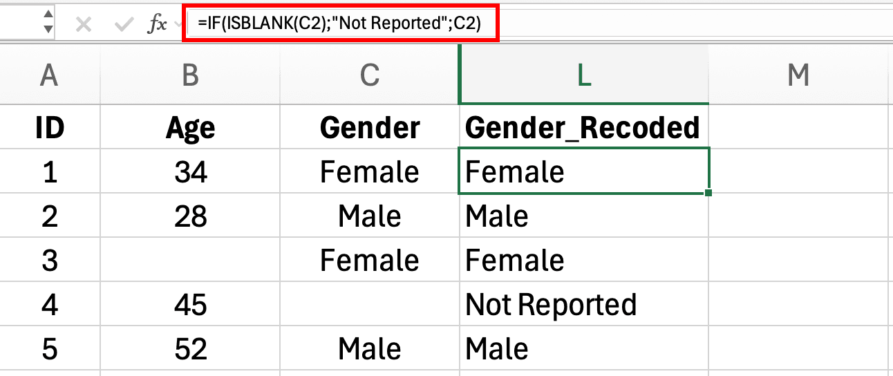
Figure 5: IF ISBLANK formula creating Not Reported category for missing Gender values in Excel

Step 2: Verify the recoding

Create a frequency table to check:

1. Select your recoded column (F2:F1000)
2. Insert > PivotTable
3. Drag your variable to Rows
4. Add Count to Values

You should see your original categories plus "Not Reported" with the count of previously missing values.

Step 3: Use in analyses

Now you can include all cases in your analyses. For example, in a chi-square test examining education differences in survey completion rates, "Not Reported" becomes a legitimate category that might reveal patterns (e.g., people who don't report education may also systematically skip other questions).

How to Interpret and Report "Missing" Category

When you create a "Missing" category, you're treating refusal to answer as a meaningful response. This requires careful interpretation in your Results section:

Example interpretation:

The "Not Reported" education category (n equals 34, 11.3%) showed significantly lower satisfaction scores (M equals 3.2, SD equals 1.4) compared to all other education levels (M equals 4.6, SD equals 1.2), t(298) equals 4.87, p less than .001. This suggests that respondents unwilling to report education level may represent a distinct subgroup with lower organizational satisfaction, possibly reflecting privacy concerns or disengagement.

APA reporting in Methods section:

Missing data on demographic variables were retained as explicit "Not Reported" categories to preserve sample size and explore potential patterns in non-response. For the education variable, 11.3% of respondents (n equals 34) did not report their education level and were retained as a separate "Not Reported" category for all analyses involving education.

Advantages and Limitations

Advantages:

• Preserves entire sample (no deletions)
• Makes missingness transparent in results
• Can reveal meaningful patterns in who doesn't respond
• Appropriate for sensitive demographic questions
• Avoids unethical imputation of categorical data

Limitations:

• Increases number of groups for comparison (may reduce power)
• Complicates interpretation (is "Not Reported" a meaningful group?)
• Can't be used in analyses requiring numeric variables
• May violate assumptions of some statistical tests
• Requires larger sample size to have adequate power with additional category

Decision Flowchart: Which Method for Your Survey Data?

Use this decision flowchart to choose the appropriate missing data method for your specific thesis scenario.

Figure 6: Missing Data Decision Flowchart - Choose the right method for handling missing data in your thesis survey analysis

Question 1: What percentage of your data is missing?

• Less than 5% → Proceed to Question 2
• 5-10% → Proceed to Question 3
• More than 10% → STOP. Consult your thesis advisor. High missingness requires advanced techniques (multiple imputation) or may indicate fundamental data collection problems.

Question 2: Is your missing data completely random (MCAR)?

Test this by comparing respondents with complete vs. incomplete data on key demographics and other variables.

• Yes, no patterns found → Use LISTWISE DELETION
• No, patterns exist → Proceed to Question 3

Question 3: What type of variable has missing data?

• Categorical (gender, education, Yes/No) → Use "MISSING" CATEGORY method
• Numeric/Scale (Likert, continuous) → Proceed to Question 4

Question 4: Will you use this variable in correlations or regression?

• Yes → Use LISTWISE DELETION (mean imputation biases correlations downward)
• No, only descriptive stats or group comparisons → Use MEAN or MEDIAN IMPUTATION

Question 5: Does your variable have outliers or is it ordinal?

• Yes (outliers present or Likert scale) → Use MEDIAN IMPUTATION
• No (approximately normal distribution) → Use MEAN IMPUTATION

Special case: Longitudinal/repeated measures data?

If you have time-series survey data where rows represent the same person at different time points:

• Consider FORWARD FILL or BACKWARD FILL
• Only if stability assumption is reasonable
• Document this clearly in Methods section

Common Thesis Scenarios and Solutions

Scenario 1: Partial Likert Scale Responses

Problem: You administered a 10-item satisfaction scale. Some respondents answered 9 items but skipped 1, leaving you with missing data on individual items.

Solution depends on purpose:

If calculating Cronbach's Alpha or scale total scores:

• Use listwise deletion at the scale level (delete cases missing any item)
• Justification: Cronbach's Alpha requires complete data on all items
• Alternative: If less than 20% of scale items are missing, calculate mean of available items as scale score

If examining individual items:

• Use median imputation (Likert scales are ordinal)
• Impute with median of that specific item, not scale mean
• Report in Methods: "For respondents missing individual scale items (n equals 14, 4.7%), missing values were replaced with the item-specific median"

Scenario 2: Demographic Data Missing

Problem: 15% of respondents didn't provide age, gender, or income information.

Solution:

For categorical demographics (gender, education):

• Create "Not Reported" category
• Never impute demographics (creates fictitious sample characteristics)
• Example: Gender becomes Male/Female/Non-binary/Not Reported

For continuous demographics (age, income):

• If using as grouping variable: Create "Not Reported" category by binning first, then adding missing bin
• If using as covariate: Use listwise deletion for analyses involving that demographic
• Never impute (misrepresents your actual sample)

Report in Methods:

Demographic variables with missing data were retained using a "Not Reported" category for gender (n equals 23, 7.6%) and education (n equals 19, 6.3%). Cases with missing age data (n equals 12, 4.0%) were excluded from analyses involving age as a variable through listwise deletion.

Scenario 3: High Dropout Rate (More than 10% Missing)

Problem: You sent a 50-question survey. Completion rate was 70%, with 30% of respondents abandoning the survey partway through.

Red flags:

• This level of missingness likely indicates survey design problems (too long, confusing, technical issues)
• Pattern is almost certainly NMAR (people who would rate lowest drop out)
• Simple Excel methods will introduce substantial bias

Solutions:

Option 1: Analyze complete vs. incomplete groups separately

• Treat survey dropout as an outcome variable
• Compare early responses between completers and non-completers - use t-tests to compare means on observed variables
• Report: "Respondents who completed the survey (n equals 210) did not differ from those who abandoned it (n equals 90) on demographic characteristics available for both groups, suggesting dropout was not systematically related to respondent profiles"

Option 2: Partial data analysis

• Use listwise deletion separately for each analysis
• Clearly report varying sample sizes
• Example: "Sample sizes varied by analysis due to listwise deletion: demographics (n equals 300), satisfaction items (n equals 210), open-ended responses (n equals 156)"

Option 3: Consult advisor about advanced techniques

• Multiple imputation - see guide for How to Import a CSV File in R to get started with R
• Pattern-mixture models
• May need to acknowledge as major limitation

Option 4: Collect more data (if possible)

• If still in data collection phase, redesign survey to reduce length
• Add progress bar, save-and-continue feature
• May be the only solution for severely compromised data

Never proceed with high-dropout data using simple mean imputation and hope reviewers don't notice. Your thesis committee will identify this immediately as a validity threat.

Scenario 4: Sensitive Questions (Income, Health, Politics)

Problem: Questions about income, mental health, political affiliation, or other sensitive topics have 20-30% non-response, far exceeding other variables.

Likely pattern: NMAR (people who would report lowest income or most stigmatized health conditions are most likely to skip)

Solution:

Use "Prefer Not to Answer" as an explicit response option during survey design (prevents this issue).

If you already have the data with missing values:

• Create "Not Reported" category
• Acknowledge this as NMAR in Methods section
• Report results for "Not Reported" group separately
• Consider this group may differ systematically from reporters

Example analysis:

Income was missing for 28.3% of respondents (n equals 85). Chi-square analysis revealed that respondents who did not report income were significantly more likely to report job dissatisfaction, χ²(1) equals 12.45, p less than .001, suggesting systematic differences between reporters and non-reporters. Therefore, income analyses are restricted to respondents who provided income information (n equals 215), with acknowledgment that findings may not generalize to the non-reporting subgroup.

This transparent approach acknowledges the limitation rather than hiding it through inappropriate imputation.

How to Report Missing Data in Your Thesis

Your thesis Methods section must include a clear, detailed subsection on missing data. This demonstrates methodological rigor and prevents committee questions during your defense. Here's how to structure it:

What to Include in Your Methods Section

1. Describe the extent of missing data

Report the percentage and number of cases with missing values, separately for each variable or set of variables.

Example:

Missing data analysis revealed varying patterns across variables. Demographic variables were largely complete, with less than 3% missing data for age (n equals 8) and gender (n equals 5). The primary outcome variable, job satisfaction, had 7.3% missing data (n equals 22), while the secondary outcome of organizational commitment had 12.1% missing (n equals 36). All predictor variables were complete with no missing values.

2. Test and report the missing data pattern

Describe whether data appears to be MCAR, MAR, or NMAR based on your diagnostic tests.

Example:

To examine whether data were missing completely at random (MCAR), respondents with complete versus incomplete data were compared on key demographics and baseline variables using independent t-tests and chi-square tests. No significant differences emerged for age, t(298) equals 0.87, p equals .39, gender, χ²(2) equals 1.45, p equals .48, education level, χ²(3) equals 2.31, p equals .51, or baseline satisfaction, t(298) equals 1.22, p equals .22. Little's MCAR test was not significant, χ²(156) equals 148.73, p equals .64, providing evidence that data were missing completely at random.

3. Justify your chosen method

Explain why you selected your specific missing data approach, with reference to the pattern diagnosed above.

Example:

Given the MCAR pattern and relatively small percentage of missing data (less than 8% for the primary outcome), listwise deletion was employed for all analyses. This approach, while reducing statistical power slightly, produces unbiased parameter estimates under MCAR assumptions (Schafer & Graham, 2002) and maintains consistency across all analyses by using the same analytic sample.

4. Report the final analytic sample

State your final sample size after applying your missing data method.

Example:

After listwise deletion, the final analytic sample consisted of n equals 264 respondents with complete data on all variables included in the primary analyses. Sensitivity analyses comparing complete cases to the full sample (N equals 300) on available baseline variables showed no systematic differences, supporting the validity of this approach.

Template for Different Methods

Listwise Deletion Template:

Missing data occurred on [X%] of cases for [variable name]. Examination of missing data patterns revealed no significant differences between respondents with complete versus incomplete data on [list demographic and key variables], suggesting data were missing completely at random. Listwise deletion was applied, resulting in a final analytic sample of n equals [X] for all subsequent analyses.

Mean/Median Imputation Template:

Missing data analysis revealed [X%] of respondents (n equals [X]) had missing values on the [variable name]. Little's MCAR test indicated data were missing completely at random, χ²([df]) equals [value], p equals [value]. To preserve statistical power while maintaining the variable's central tendency, mean imputation was applied, replacing missing values with the sample mean of M equals [X] (SD equals [X]). Sensitivity analyses comparing results with and without imputation showed consistent patterns, supporting this approach.

Missing Category Template:

Demographic variables with missing data were retained using explicit "Not Reported" categories: [X%] for gender (n equals [X]), [X%] for education (n equals [X]). This approach preserves the full sample and allows examination of potential non-response patterns. Respondents who did not report demographics did not differ significantly from those who did on key outcome variables, suggesting non-response was not systematically related to study outcomes.

Common Committee Questions (and How to Address Them)

Question: "Why didn't you use multiple imputation?"

Answer: "Multiple imputation is the gold standard for handling missing data, particularly with MAR or NMAR patterns. However, given our data were missing completely at random, shown by Little's MCAR test (p equals .64), and the missingness was less than 8%, listwise deletion provides unbiased estimates with greater simplicity and transparency. Multiple imputation would have required software beyond Excel and added complexity without improving estimate quality under MCAR conditions."

Question: "How did you determine the data were MCAR?"

Answer: "I conducted several diagnostic tests: First, I compared respondents with and without missing data on all observed demographics and baseline variables using t-tests and chi-square tests. No significant differences emerged. Second, I calculated Little's MCAR test, which was non-significant (p equals .64), failing to reject the null hypothesis that data are MCAR. Third, I examined missing data patterns visually and found no systematic clusters. While these tests cannot prove MCAR definitively, they provide strong evidence supporting the MCAR assumption."

Question: "Didn't you lose statistical power by deleting cases?"

Answer: "Yes, listwise deletion reduced my sample from 300 to 264, a 12% reduction. However, post-hoc power analysis using G*Power showed that with n equals 264, I still achieved power of 0.87 for detecting medium effect sizes (d equals 0.5) at alpha equals .05. This exceeds the conventional threshold of 0.80, indicating adequate power for my primary analyses. The alternative approaches (mean imputation) would have preserved sample size but introduced different biases, particularly for correlation and regression analyses."

Frequently Asked Questions

Next Steps: Using Missing Data Methods in Your Thesis

You now have a complete framework for handling missing data in Excel survey analysis. The key to thesis success is not avoiding missing data (impossible in real research), but handling it transparently and appropriately for your specific scenario.

Before finalizing your approach:

1. Diagnose your missing data pattern using the tests described in this guide. Don't assume it's random.

2. Choose the method that matches your pattern and variable type using the decision flowchart. Different variables may require different approaches.

3. Document everything in your Methods section. Your committee needs to see that you made informed, defensible decisions.

4. Run sensitivity analyses comparing results with different missing data methods. If conclusions don't change, you have evidence of robustness.

5. Consult your advisor if you have more than 10% missing data or evidence of NMAR patterns. Some situations require advanced techniques beyond Excel.

Missing data doesn't have to derail your thesis. With the right approach, you can produce valid, defensible results even with imperfect data.

For your next steps in survey analysis, learn how to report your descriptive statistics in APA format or review common mistakes in survey analysis to avoid other validity threats.

References

American Psychological Association. (2020). Publication Manual of the American Psychological Association (7th ed.). American Psychological Association.
Schafer, J. L., & Graham, J. W. (2002). Missing data: Our view of the state of the art. Psychological Methods, 7(2), 147-177.
Little, R. J. A., & Rubin, D. B. (2019). Statistical Analysis with Missing Data (3rd ed.). Wiley.
Enders, C. K. (2010). Applied Missing Data Analysis. Guilford Press.