This step-by-step tutorial shows you how to perform moderation analysis in AMOS Graphics using a practical case study with real data.
You'll learn how to standardize variables in SPSS, compute interaction terms, build structural equation models in AMOS, and interpret your moderation results. Moderation analysis (also called moderated multiple regression or MMR) is a statistical technique that tests whether a third variable affects the strength or direction of the relationship between your independent and dependent variables.
You can also perform moderation analysis using Ordinary Least Squares (OLS) regression in SPSS alone. However, if you're working with AMOS models, you'll need to standardize all quantitative variables in SPSS first to reduce multicollinearity issues.
To complete this tutorial you will need SPSS Statistics and AMOS installed on your computer.
What Is Moderation Analysis?
When researching a particular phenomenon involving the interaction between two or more variables, we want to get relevant results that apply to the real world.
Though many external factors can affect how two variables relate, it would be impossible to include all of them in a single study. However, we can identify those factors of high relevance for our case and investigate if they have an effect or moderate the relationship between two variables.
In statistics, moderation analysis refers to the process of testing the effects of a moderator variable (Mo) on the relationship between an independent variable (X) and a dependent variable (Y).
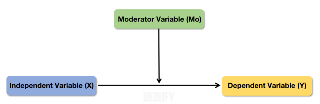 Figure 1: Moderator variable (Mo) affects the relationship between independent variable (X) and dependent variable (Y).
Moderator variables, also known as interaction variables, can be both quantitative (numeric values: age, weight, test score, etc.) or qualitative (non-numeric values: gender, education, social status, etc.).
If the variables in your study are quantitative, they need to be computed as a mean center (average of all values) before conducting the moderation analysis in AMOS. This not only makes interpretation easier but also reduces potential multicollinearity issues with the model when multiple variables are present.
Multicollinearity can make the estimates very sensitive even to the smallest change in the model due to an increase in the variance of the coefficient estimates.
Moderation Analysis In AMOS [Case Study]
Let’s assume we investigate if financial regulation has a moderating effect on the relationship between financial investment and risk.
In this case, regulation is the moderator variable (Mo), investment is the independent variable (X), and risk is the dependent variable (Y). In other words, we will investigate the moderating effects of regulation on the relationship between investment and risk.
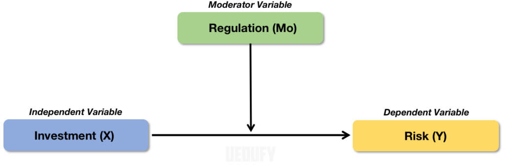 Figure 2: Moderation analysis conceptual model: Regulation moderates the investment-risk relationship.
To follow along with this tutorial, download the sample dataset from the sidebar. This is a dummy dataset for educational purposes only.
Alternatively, you can use your own dataset or create a new one by generating random numbers in Excel and importing the Excel file in SPSS Statistics.
Prepare Your Data in SPSS
Import A Data Set In SPSS
Before we proceed with the moderation analysis in AMOS, we need to mean center the values for the quantitative variables used in our study.
Unzip and double-click on the SPSS raw sample file (Moderator Analysis SPSS Sample.sav) downloaded earlier. The imported sample dataset in SPSS should look like the capture below.
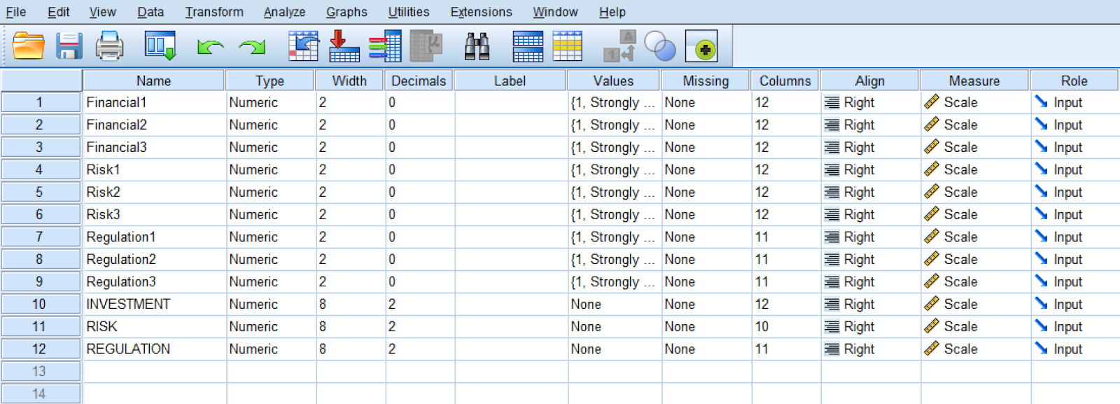 Figure 3: SPSS Variable View with the case study dataset variables.
Where:
-
Financial1-3 are the Financial Investment variables (quantitative)
-
Risk1-3 are the Financial Risk variables (quantitative)
-
Regulation1-2 are the Financial Regulation variables (quantitative)
-
INVESTMENT is the independent variable (X) computed from the Financial1-3 variables.
-
RISK is the dependent variable (Y) computed from the Risk1-3 variables.
-
REGULATION is the moderator variables (W) computed from the Regulation1-2 variables.
From here onwards, our focus will be on the computed variables (INVESTMENT, RISK, and REGULATION) only.
To import your own data set in SPSS, on the top menu go to File → Import Data → Excel. On the Open Data window, navigate to the location where the Excel file is located on your disk, select the file and click the Open button.
Create Standardized Values For Variables In SPSS
To avoid multicollinearity issues with the model, we should create standardized values for the independent, dependent, and moderator variables in our example.
In the SPSS Statistics top menu, navigate to ** Analyze → Descriptive Statistics → Descriptives.
In the Descriptives window, move the INVESTMENT, RISK, and REGULATION variables by selecting each variable on the left box and clicking on the arrow button in the center to move it to the right.
Make sure the Save standardized values as variables checkbox is checked. Press the OK button to proceed to create the standardized values for the selected variables.
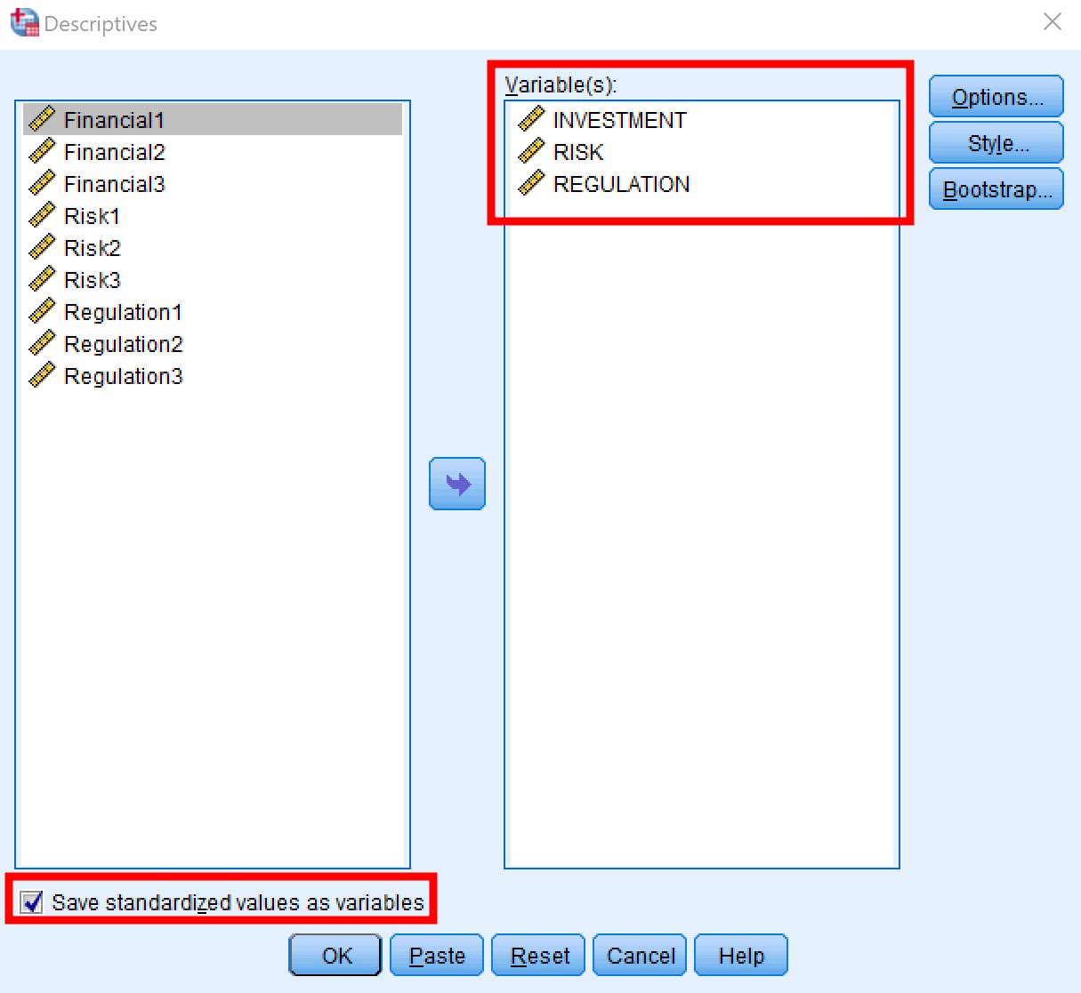 Figure 4: SPSS Descriptives dialog with Save standardized values checked.
This will create three new standardized variables respectively ZINVESTMENT, ZRISK, and ZREGULATION.
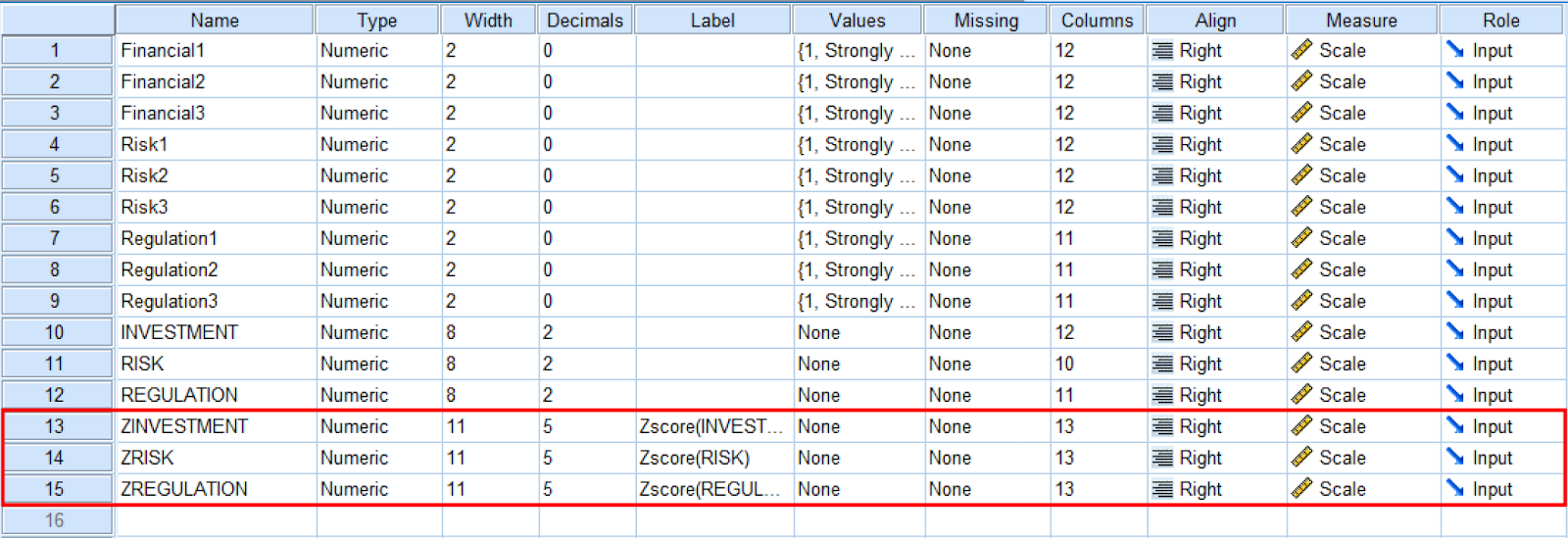 Figure 5: Standardized variables created in SPSS (ZINVESTMENT, ZRISK, ZREGULATION).
Compute Values For Interaction Variable
Next, we need to compute values for the interaction variable by calculating the product between the independent variable and the moderator variable.
On the SPSS top menu, navigate to Transform → Compute Variable.
In the Compute Variable window:
[1] Type a name (e.g., INTERACTION) in the Target Variable box.
[2] Select the independent variable (ZINVESTMENT) in the left box and use the arrow button to move it to the Numeric Expression box.
[3] Click on the multiply (*) button in the calculator.
[4] Add the moderator variable (ZREGULATION) to the Numeric Expression box.
[5] Click OK to compute the interaction variable.
Here is a graphical representation of these steps.
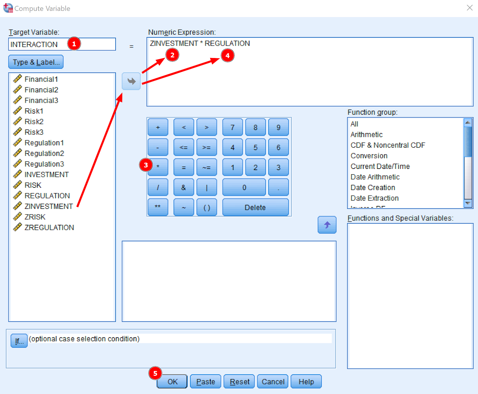 Figure 6: Compute Variable dialog in SPSS for computing the interaction term (ZINVESTMENT * ZREGULATION).
Note that we only use standardized variables to compute the interaction (moderator) variable.
Save A Data Set In SPSS
The final step in SPSS is to save our work so that all new variables will appear in AMOS. To do so, navigate to File → Save As, give a name to the new data set, and click the Save button.
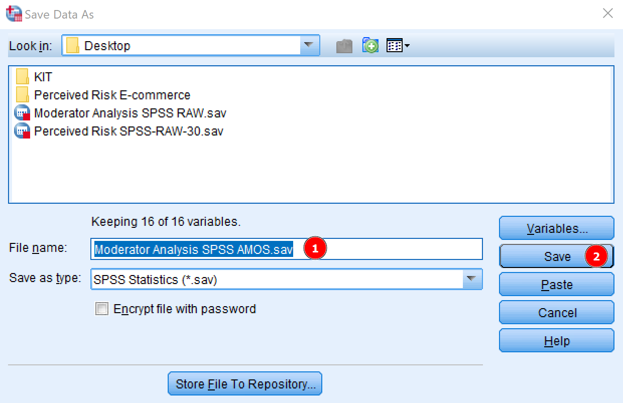 Figure 7: Save Data As dialog in SPSS to save the dataset with new variables.
Now we are ready to conduct a moderation analysis in AMOS using our sample SPSS data set.
Build the Moderation Model in AMOS
Import SPSS Data Set In AMOS
Launch Amos. The first thing we need to do is to import the new SPSS data set into AMOS. To do so, click on the Select Data File icon on the icons panel.
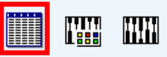 Figure 8: Select Data File icon in the AMOS toolbar.
On the Data Files window, click the File Name button and navigate to the location you saved the SPSS file earlier (Step 4). Select the file and click Open.
To finish the import, click OK on the Data Files window.
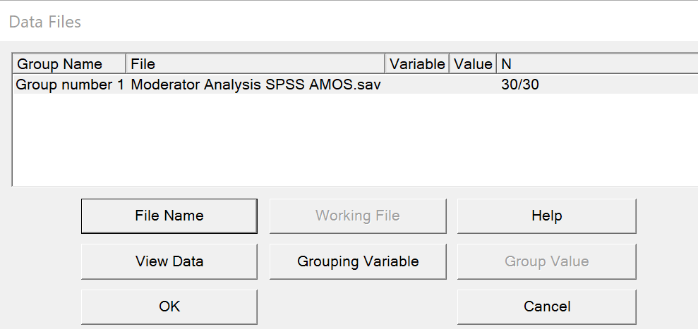 Figure 9: Data Files dialog in AMOS with the SPSS dataset imported.
Create A Model In AMOS
To create the model for our case study in AMOS, first, click on the List variables in data set icon to visualize all the variables in the data set.
 Figure 10: List variables in data set icon in AMOS.
Drag and drop the independent, moderator, and interaction variables on the left side of the working space, and the dependent variable on the right side similar to how is shown in the capture below. Don’t worry about aesthetics for now. We will fix that in a moment.
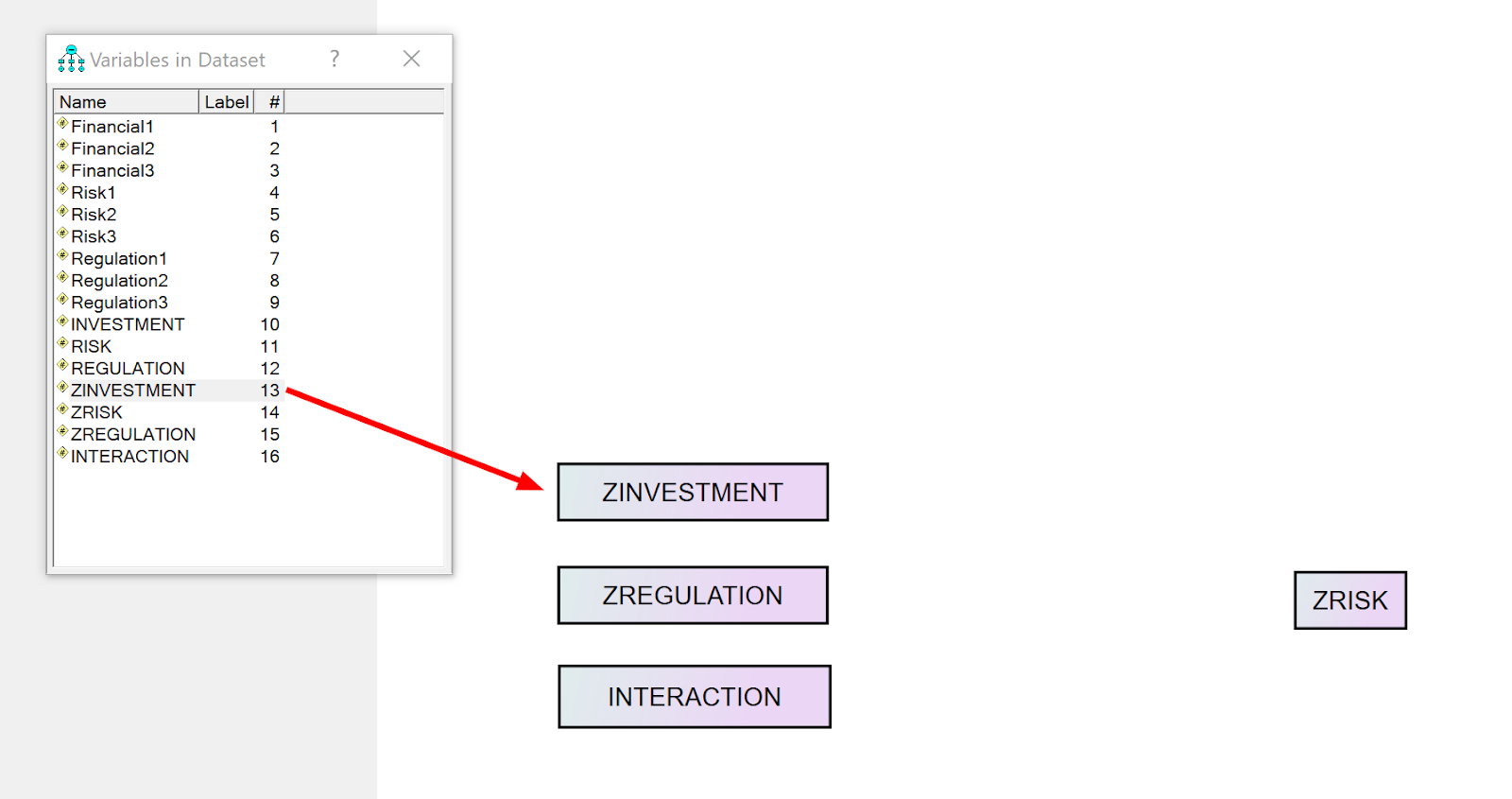 Figure 11: Variables dragged from the variable list to the AMOS workspace.
Establish Cause and Effect Relationship
To establish the cause and effect relationship between the variables in our study, first, click on the Draw paths (single-headed arrows) icon.
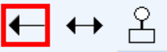 Figure 12: Draw paths (single-headed arrows) icon in AMOS.
In this example, all predictor variables representing the cause are located on the left side while the effect predicted variable is on the right side of the workspace.
Draw arrows from all the predictors (ZINVESTMENT, ZREGULATION, INTERACTION) pointing to the predicted variable (ZRISK). The model for this case study should look like this in AMOS:
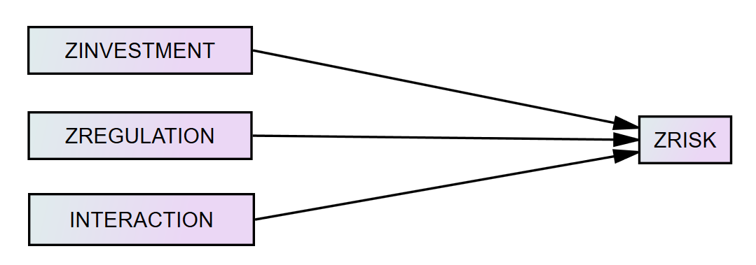 Figure 13: Path model with single-headed arrows from predictors to ZRISK.
Establish Covariance Between Predictors
Covariance is used to determine the relationship between the predictor variables in our model. In AMOS, to establish covariance between predictors, first, click on the Draw covariance (double-headed arrows) icon.
 Figure 14: Draw covariance (double-headed arrows) icon in AMOS.
Next, draw covariance between ZINVESTMENT, ZREGULATION, and INTERACTION variables.
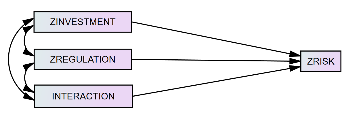 Figure 15: Covariances (double-headed arrows) established between ZINVESTMENT, ZREGULATION, and INTERACTION.
Add Residual (Error) To Predicted Variable
Similarly, with the OLS analysis, the residual (error) is used to show the difference between the predicted and observed actual value. In other words, how far vertically the data points are from the regression line.
To add residual (error) in AMOS, select on the Add a unique variable to an existing variable icon.
 Figure 16: Add a unique variable to an existing variable icon in AMOS.
Click on the predicted variable (ZRISK).
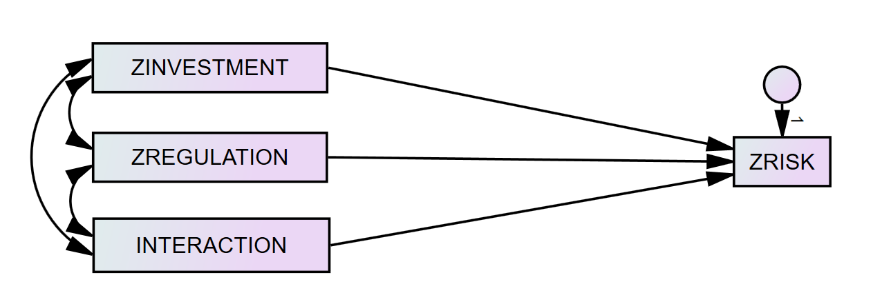 Figure 17: Residual error variable added to ZRISK (unnamed).
Finally, we need to add a name for the error. The easiest way is to instruct SPSS to name it by navigating to **Plugins → Name Unobserved Variables. SPSS named the residual variable in this case “e1” as seen below.
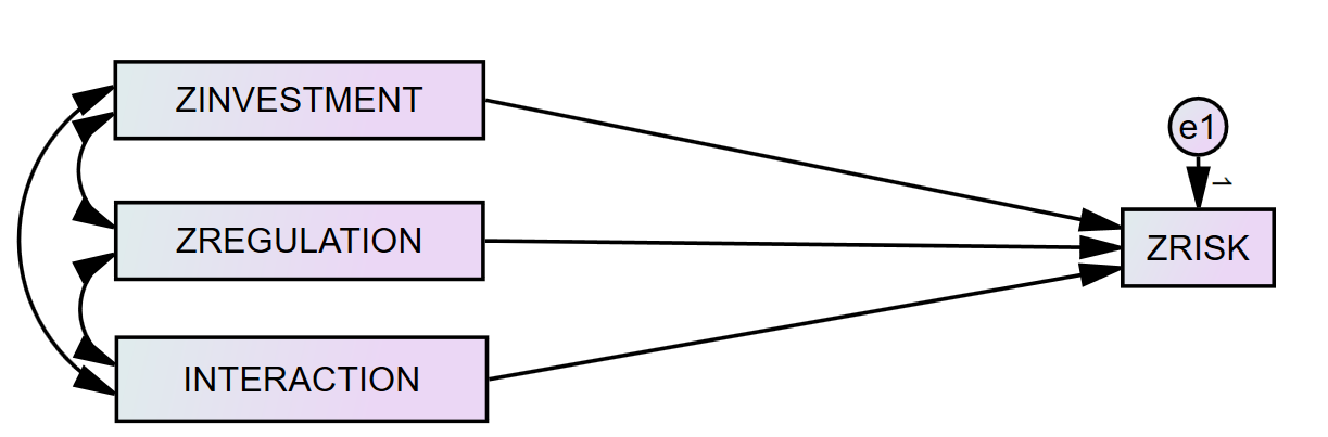 Figure 18: Complete moderation model in AMOS with the e1 residual error named.
Touch Up Your Model
Before we proceed with the moderation analysis in Amos, let’s work on the aesthetics of your diagram. Amos provides us with a few tools accessible via the icon panel and listed in the following diagram.
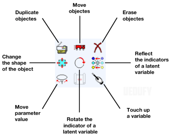 Figure 19: AMOS toolbar tools for moving, duplicating, rotating, and formatting objects.
In most cases, you will need to move objects, change the shape of the object, duplicate objects, and erase objects.
To quickly fix a messy diagram, use the touch-up a variable (wand) tool and click on all the shapes in your model. AMOS will quickly align everything and make your diagram look much better.
You can change the colors, font size, style, etc., via the Object Properties window, which is accessible by double-clicking on any object in the workspace.
Run the Analysis and Interpret Results
Change Analysis Properties For The Output File
Before we proceed with the moderation effect in AMOS, we need to change some of the properties of the output file. Navigate to View → Analysis Properties, click on the Output tab and mark the following checkboxes:
-
Minimization history
-
Standardized estimates
-
Squared multiple correlations
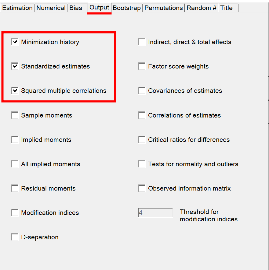 Figure 20: Analysis Properties Output tab with the required checkboxes selected.
Close the Analysis Properties window.
Save Model In AMOS
To save your model, go to File → Save As, type a file name, and press the Save button. Your Amos file will have the .amw extension.
Run Moderator Analysis In AMOS
Finally, we are ready to run a moderation analysis in AMOS. To proceed, navigate to ** Analyze → Calculate Estimates** or simply press the CTRL+F9 combination.
Amos will conduct the analysis and populate the model with estimates.
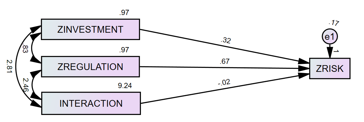 Figure 21: Model with standardized estimates: ZREGULATION (.67) is the strongest predictor of ZRISK.
Moderation Analysis Results In AMOS
Once the analysis is completed, navigate to View → Text Output or simply press the F10 key on your keyboard to check the moderation analysis results.
On the AMOS Output window, click on Estimates. The moderating effects for the interaction variable will be listed under the Regression Weights.
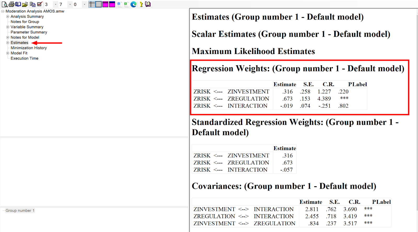 Figure 22: Regression Weights table in AMOS Output showing estimates, standard errors, and p-values.
Interpreting Moderation Analysis Results
Before we dive into analyzing the results, please note that AMOS is a piece of software designed for other types of analysis [Confirmatory Factor Analysis (CFA), Structural Equation Modeling (SEM), Path Analysis, etc.) and is not really suitable for moderation analysis.
If you are looking into finding the levels of conditional effects of the focal predictor, look into moderation analysis using PROCESS Macro in SPSS as a more suitable solution.
Looking at the P column we can observe that the interaction effect of the INTERACTION variable on ZRISK is 0.802 (P > 0.05) therefore not statistically significant. The probability of getting a critical ratio as large as 0.251 in absolute value is 0.802. In other words, the regression weight for INTERACTION in the prediction of ZRISK is not significantly different from zero at the 0.05 level (two-tailed).
Similarly, ZINVESTMENT has no effect on ZRISK respectively 0.220 (P > 0.05) and therefore not statistically significant either. The probability of getting a critical ratio as large as 1.227 in absolute value is 0.220. In other words, the regression weight for ZINVESTMENT in the prediction of ZRISK is not significantly different from zero at the 0.05 level (two-tailed).
However, we can see that the relationship between ZREGULATION and ZRISK is statistically significant (P < 0.05). In other words, the regression weight for ZREGULATION in the prediction of ZRISK is significantly different from zero at the 0.001 level (two-tailed).
In conclusion, the interaction effect of regulation on financial risk is not statistically significant in this case study.
Note that in this example we are using a small sample size with fictitious values for educational purposes only. A larger dataset might provide different results.
Frequently Asked Questions
Wrapping Up
Conducting a moderation analysis in AMOS is a relatively simple process that helps us test if a moderation variable has an effect on the relationship between a dependent and independent variable in the regression.
Though AMOS is mostly known for its use in Structural Equation Modeling (SEM), confirmatory factor analysis, covariance, and path analysis, its powers go well beyond its fame. This lesson is just one such example.
References
Aguinis, H. (2004). Regression analysis for categorical moderators. Guilford Press.