Learn how to run and interpret repeated measures ANOVA in SPSS with this step-by-step tutorial. We'll walk through a complete analysis using real data, from checking assumptions to interpreting SPSS output tables and reporting results in APA format.
This guide covers everything you need: when to use repeated measures ANOVA, how to handle sphericity violations (Mauchly's Test, Greenhouse-Geisser correction), interpret within-subjects effects, and run pairwise comparisons. Download the practice dataset from the sidebar (password: uedufy) and follow along to master this essential statistical test for analyzing repeated measurements.
What You'll Learn
By the end of this tutorial, you'll be able to:
-
Know when to use repeated measures ANOVA for one-way and two-way.
-
Understand the assumptions of repeated measures ANOVA.
-
Perform one-way ANOVA for repeated measures in SPSS using the between-subjects and within-subject factors.
-
Interpret the repeated measures ANOVA results in SPSS
Get a cup of coffee or tea and let’s learn something new today!
When To Use One-Way Repeated Measures ANOVA
Use one-way repeated measures ANOVA when you want to compare the mean scores of the same group of participants measured at three or more different time points or under three or more different conditions.
Unlike the t-test (which compares means between two groups or two time points), repeated measures ANOVA handles multiple measurements from the same participants.
Requirements for One-Way Repeated Measures ANOVA:
Your study should have these characteristics:
-
one group of respondents measured using the same scale on three or more different periods OR each participant measured using at least three different items (e.g., questions) using the same response scale.
-
One categorical independent variable (also known as a repeated factor).
-
One continuous dependent variable is used to repeat observations also known as a repeated measure.
Confused? Let's fix that by looking to a repeated measure design case study next.
Assuming we want to test the efficacy of two weight-loss diet programs (e.g., low-carb and low-fat), and 3 repeated periods: 1st Period (before starting the diet); 2nd Period (after 30 days), and 3rd Period (after 90 days).
We can design this study to include 50 participants, divided into two groups of 25 participants each. A participant can be part of one group only and only one diet program will be applied to each group.
Here's how the dataset for this case study looks in the SPSS Data View tab:
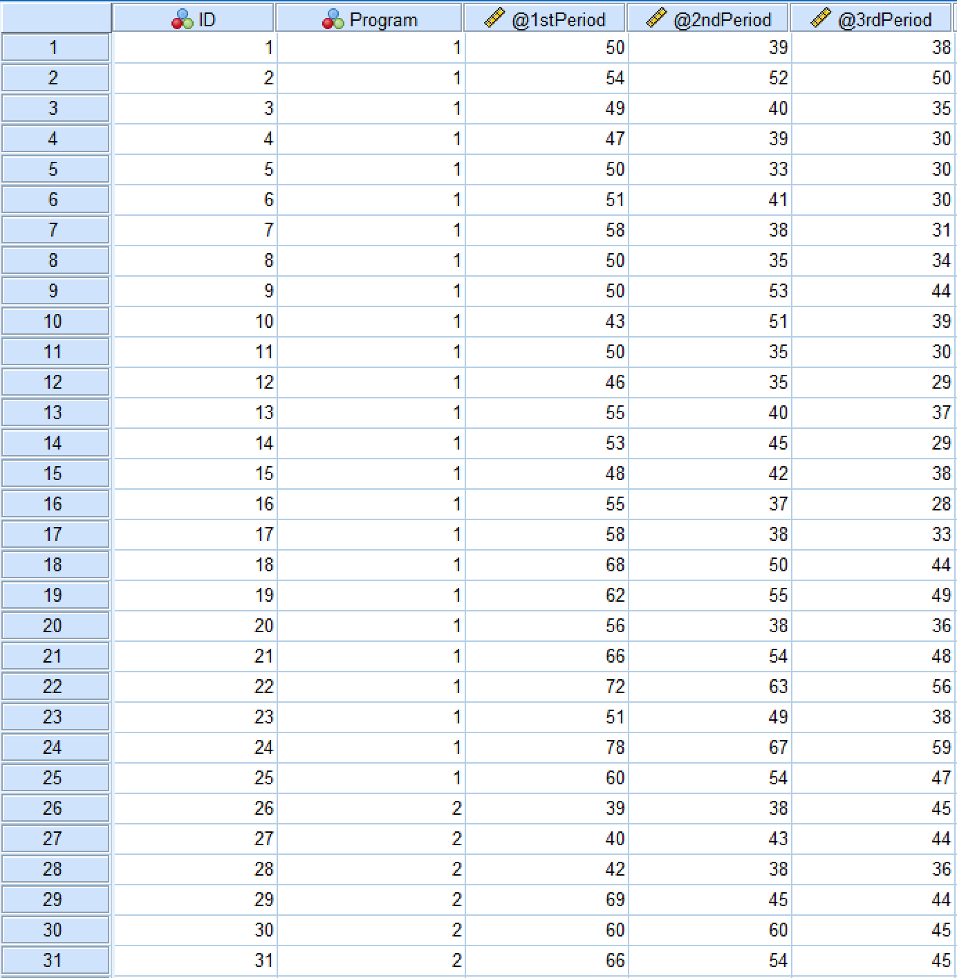
Figure 1: SPSS Data View showing the repeated measures dataset structure
And here is the Variable View tab in SPSS:
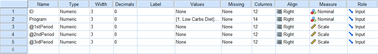
Figure 2: Variable View showing variable definitions for repeated measures ANOVA
The independent variable in this example is the [diet] Program which consists of two levels: low-carb and low-fat diets. The dependent variable is 1st Period, 2nd Period, and 3rd Period. We also have the ID where each respondent in the study is associated with a unique number.
Since this study has one independent variable and we plan to measure the diet effects for the same participants in two different groups across three time periods, the one-way ANOVA for repeated measures would be the right approach.
Repeated Measures ANOVA Assumptions
Before running repeated measures ANOVA, verify your data meets these key assumptions:
1. Independence of Observations
All observations must be independent - each participant can only belong to one group, and participants cannot influence each other's responses.
How to check: Verify your research design ensures participants are independent. This is a design issue, not tested statistically.
2. Sphericity (Equality of Variances)
The variances of the differences between all possible pairs of within-subjects conditions must be equal.
How to check in SPSS: Mauchly's Test of Sphericity (SPSS calculates this automatically)
- If p > .05: Assumption met, use standard F-test
- If p < .05: Assumption violated, use Greenhouse-Geisser or Huynh-Feldt correction
3. Normality
The dependent variable should be approximately normally distributed for each level of the within-subjects factor.
How to check in SPSS:
- Visual inspection: Q-Q plots, histograms
- Statistical test: Shapiro-Wilk test for each time point
- For large samples (n > 30), ANOVA is robust to minor violations
Important: Repeated measures ANOVA is fairly robust to violations of normality, especially with larger sample sizes (n > 30).
Now that you understand the assumptions, let's run the analysis in SPSS!
Perform One-Way ANOVA For Repeated Measures in SPSS [Practice]
Import the dataset you downloaded earlier in SPSS by navigating to Open → Data and selecting the .sav file or simply double-click on the .sav file to automatically open it in SPSS.
Here are the steps to conducting one-way repeated measures ANOVA analysis in SPSS:
-
Navigate to Analyze → General Linear Model → Repeated Measuresin the SPSS top menu.
-
On the Repeated Measure Define Factor(s) window, specify:
-
The Within-Subject Factor Name, e.g., Period or Time Frame.You can rename the name with something appropriate in the case is needed.
-
The Number of Levels respectively the number of dependent variables in the study. In our case, this is three.
-
Click the Add button to move the factor and the defined variables into the respective box.
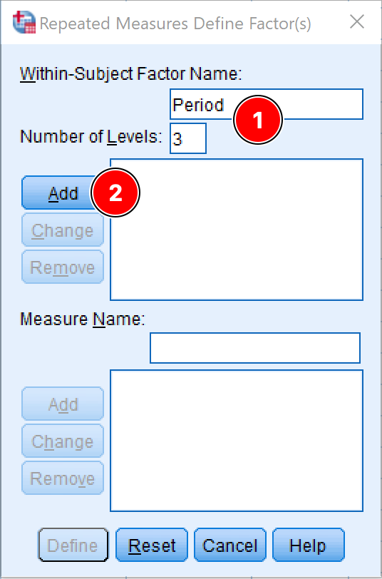
Figure 3: Defining the within-subject factor for repeated measures ANOVA
- Click the Define button.
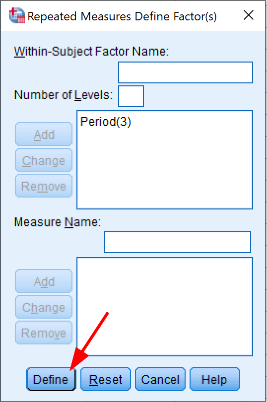
Figure 4: Clicking Define to proceed with repeated measures ANOVA setup
- In the Repeated Measures window, specify the dependent variables in the correct order for each Within-Subjects Variables position.
In our SPSS sample dataset, we have three dependent variables representing three periods: 1st Period, 2nd Period, and 3rd Period.
Assign each variable to its corresponding position:
- 1st Period → position (1)
- 2nd Period → position (2)
- 3rd Period → position (3)
You can select each variable and use the arrow button to move it to the appropriate box, or simply drag and drop each dependent variable to its position.
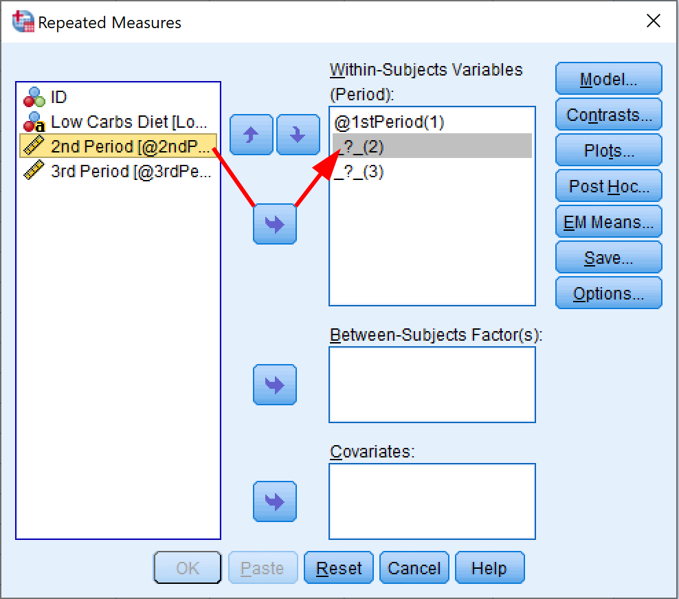
Figure 5: Adding within-subjects variables for repeated measures ANOVA
- Add the independent variable of interest to the Between-Subject Factor(s) box. In our case, the independent variable is the Program.
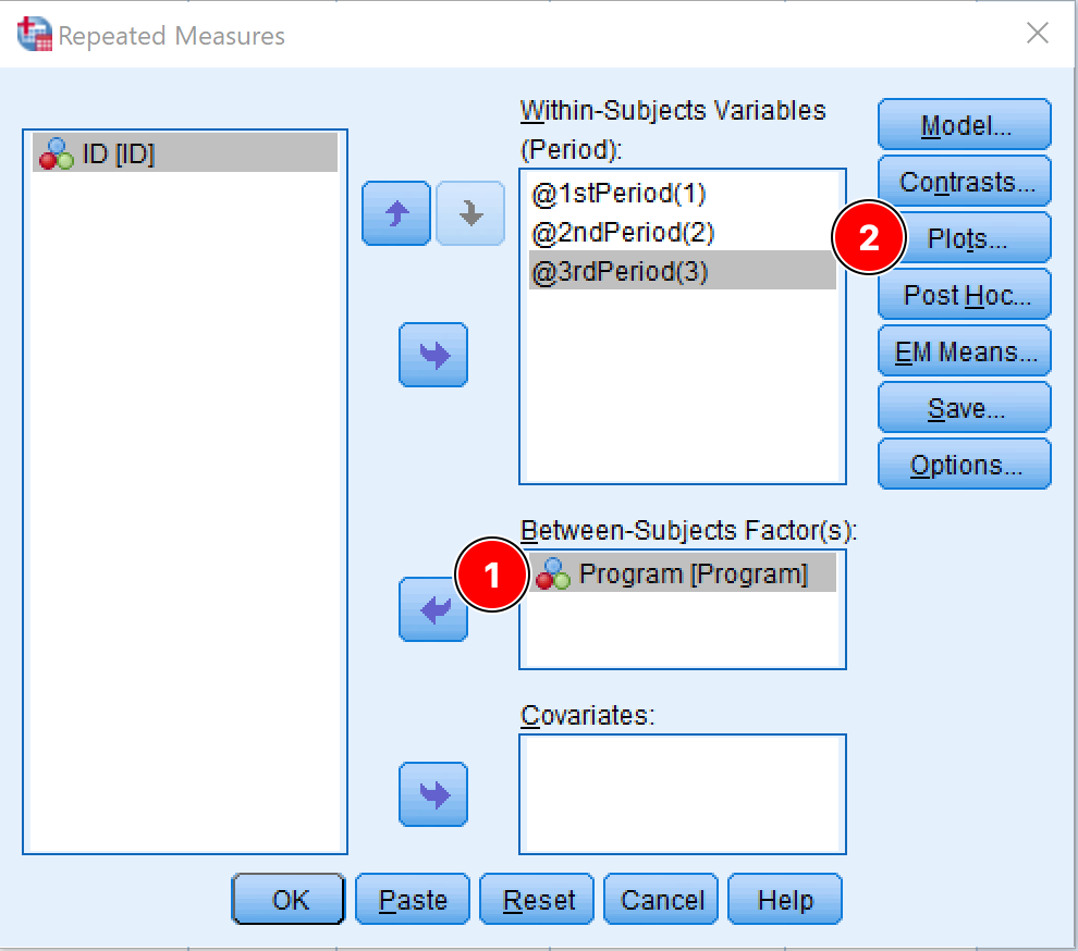
Figure 6: Adding the between-subjects factor (Program) in SPSS
Before we proceed with the one-way ANOVA for repeated measures in SPSS, we need to change some settings for the analysis. Click on the Plots button.
- On the Profile Plots window, move the independent factor (Program) to the Horizontal Axis box, and the dependent factor (Period) to the Separate Lines box. Click the Add button.
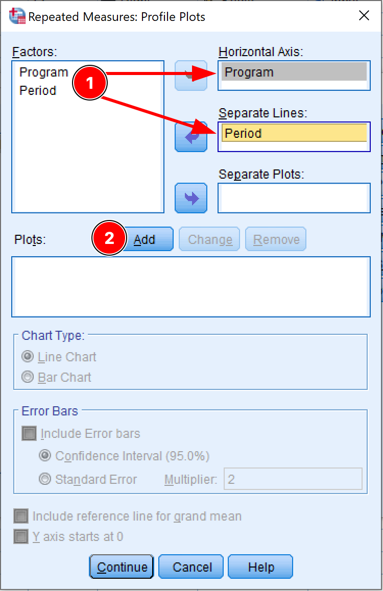
Figure 7: Setting up profile plots for repeated measures ANOVA
The Plots box will get populated. For instance, for our dataset, the plot should be Program*Period as in the picture below.
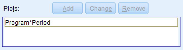
Figure 8: Confirming the Program*Period interaction plot has been added
Click Continue. You should be back at the Repeated Measures window.
Since we only have two levels for the independent variable (Low Carbs and Low Fat Diets) we do not need to run the Post Hoc test (also known as the multiple comparison test). However, if the ANOVA for repeated measures analysis consists of three or more groups, a Post Hoc test is necessary to investigate which groups' mean is different and control the familywise error rate. This is only the case when the ANOVA P-value is significant for the means of all groups.
-
Next, click on the EM Means (Estimated Marginal Means) button. Here we need to adjust the following settings:
-
We want to see the means for the dependent variable so move the Period to the Display Means box.
-
Check the Compare main effects checkbox.
-
Select the Bonferroni on the Confidence interval adjustment drop-down menu.
The Bonferroni correction is the simplest way to control the risk of encountering the type I error (false-positive) and rejecting the null hypothesis when it is actually true.
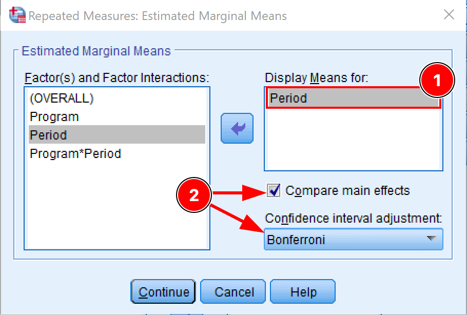
Figure 9: Configuring estimated marginal means with Bonferroni correction
Click Continue to save the settings and exit the EM Means window.
-
[Optional] Once on the Repeated Measures window, click on the Options button and make sure the following checkboxes are checked:
-
Descriptive statistics
-
Estimates of effect size
-
Homogeneity tests
Click Continue to save the settings and exit the Options window.
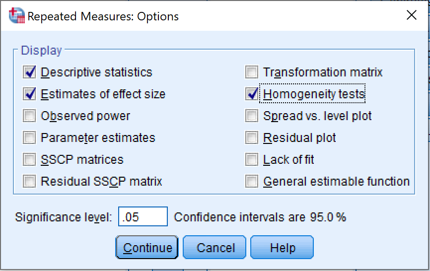
Figure 10: Selecting display options for repeated measures ANOVA output
- Finally, on the Repeated Measures window, click OK to proceed with the ANOVA for repeated measures analysis in SPSS.
Interpret ANOVA for Repeated Measures Output in SPSS
- The first table in the ANOVA repeated measures output is Within-Subjects Factors which is represented by three periods, respectively 1st Period, 2nd Period, and 3rd Period in our example.
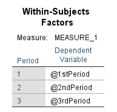
Figure 11: Within-Subjects Factors output table in SPSS
- The Between-Subjects Factors table shows the treatments (conditions) applied to the subjects. In our examples, these conditions are Low Carbs Diet and Low Fat Diet. We can also observe that the population N is equal for both treatments (N = 25 subjects).
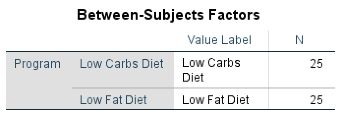
Figure 12: Between-Subjects Factors output showing equal group sizes
- In the Descriptive Statistics table we can see that the mean is overall higher in the 1st Period (Total Mean = 54.76), followed by the 2nd Period (Total Mean = 45.74) and 3rd Period (42.16) which can indicate a link between the diet programs and weight loss of the participants.
Moreover, when we look at the mean between the groups for each diet program, we can observe that the mean for Low Carbs Diet group is lower than that of the Low Fat Diet group which may indicate that a low carbs diet program is more efficient – with the exception of 1st Period where the means between the two programs are the closest.
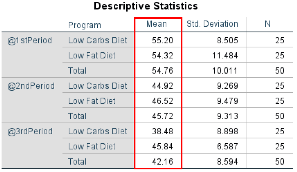
Figure 13: Descriptive statistics showing means and standard deviations for each group and time period
- The Box's Test of Equality of Covariance Matrices (also known as Box's M Test) is a parametric test for comparing variability in multivariate samples. This test explicitly checks to see whether two or more covariance matrices are homogeneous (equal).
As seen in the output below, the Box's Test result is 14.961, and the Significance P-value is 0.030. It is important to keep in mind that the Box's Test α level is 0.01 (Significant if < 0.01). Therefore we have a Box's Test that has a non-statistically significant output of 0.030. Therefore, we fail to reject the null hypothesis and meet the equal population covariance matrices assumption.
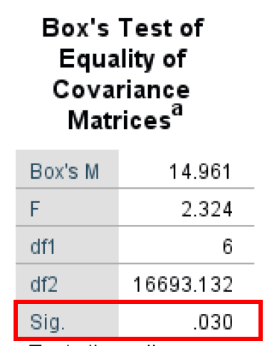
Figure 14: Box's M Test output assessing equality of covariance matrices
- The Multivariate Test shows us the overall mean difference in the repeated measures. The multivariate test implies observational independence and multivariate normality. One advantage of using the Multivariate Test is that it does not imply sphericity, as the univariate approach does – as the case in this example.
The Multivariate Test is conducted using four different test statistics (Pillai's Trace, Wilks' Lambda, Hotelling's Trace, and Roy's Largest Root) which provide basically the same information. The most important metric here is the P-value (Sig. column) with values across all statistical tests for Period and Period*Program of 0.000 therefore statistically significant (Significant if < 0.05)
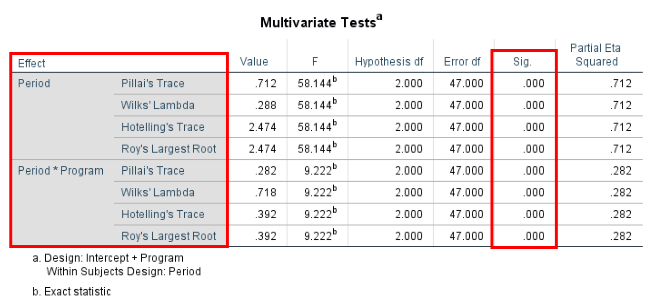
Figure 15: Multivariate test statistics for repeated measures ANOVA
- Mauchly’s Test of Sphericitytest determines if the variances between all differences between all possible pairs of groups are equal (whether the sphericity assumption is violated or not).
The Mauchly's Test has anα level of 0.05 and to meet the sphericity assumption we need to have a value greater than that. In our case, the calculated P-value is 0.02 therefore we are not meeting the sphericity assumption.
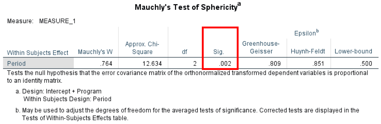
Figure 16: Mauchly's Test checking sphericity assumption
- The Tests of Within-Subjects Effects test determines if there were any significant differences between means at any point in time. As with the previous tests, the Sphericity Assumed has an α level of 0.05, and a P-value < 0.05 shows statistical significance.
In our case, we can assume sphericity for both Period and Period*Program.
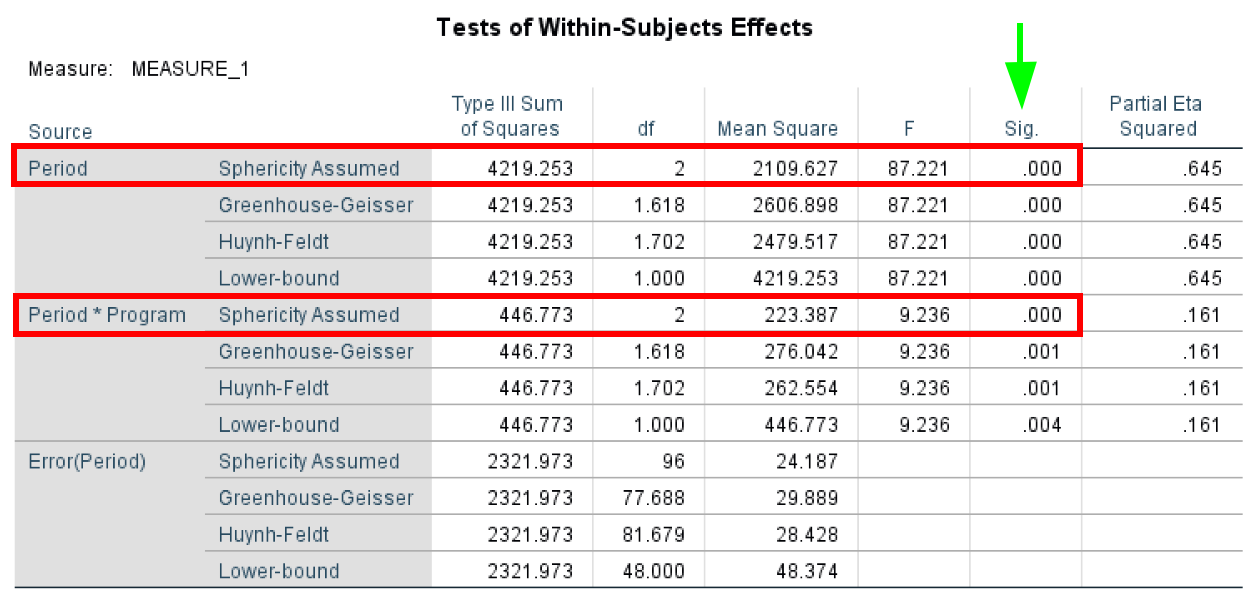
Figure 17: Within-Subjects Effects showing significant main effect of time
- The Tests of Within-Subjects Contrasts test determines if there was a statistically significant change between the means at various time points and is useful when performing trend analysis. The Tests of Within-Subjects Contrasts has an α = 0.05. In our case study, we can see that Period and Period*Program are statistically significant with P-values < 0.05 as highlighted in the table below.
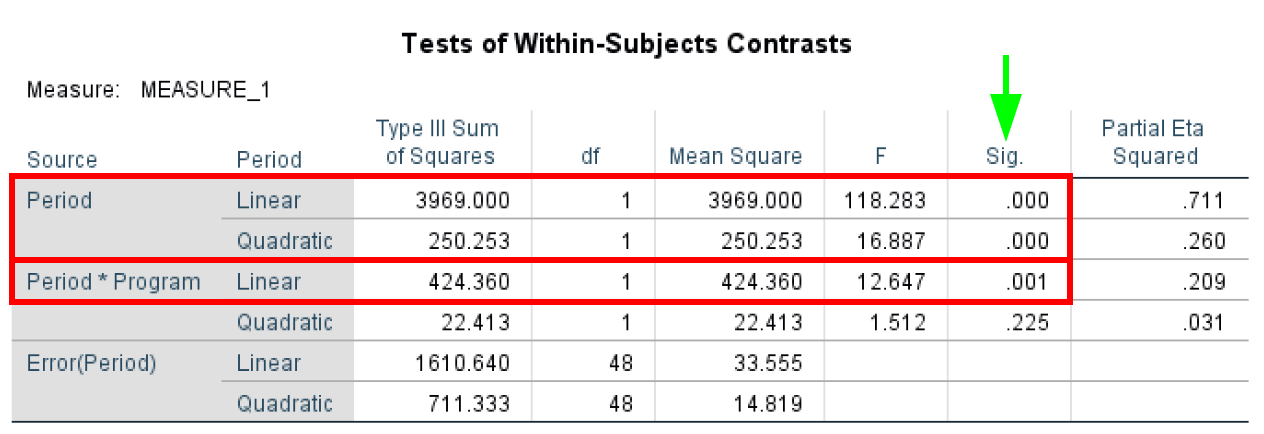
Figure 18: Within-Subjects Contrasts for trend analysis
- Levene's Test of Equality of Error Variances tests the homogeneity of variance by comparing the variances of two or more groups given a variable. Levene's Test of Equality of Error Variances has an α level of 0.05 where any P-value lower than 0.05 violates the homogeneity of variance assumption.
Looking at Levene’s Test of Equality of Error Variance output for our case study, we can see that all P-values are >0.05 therefore we do not violate the assumption of homogeneity of variance.
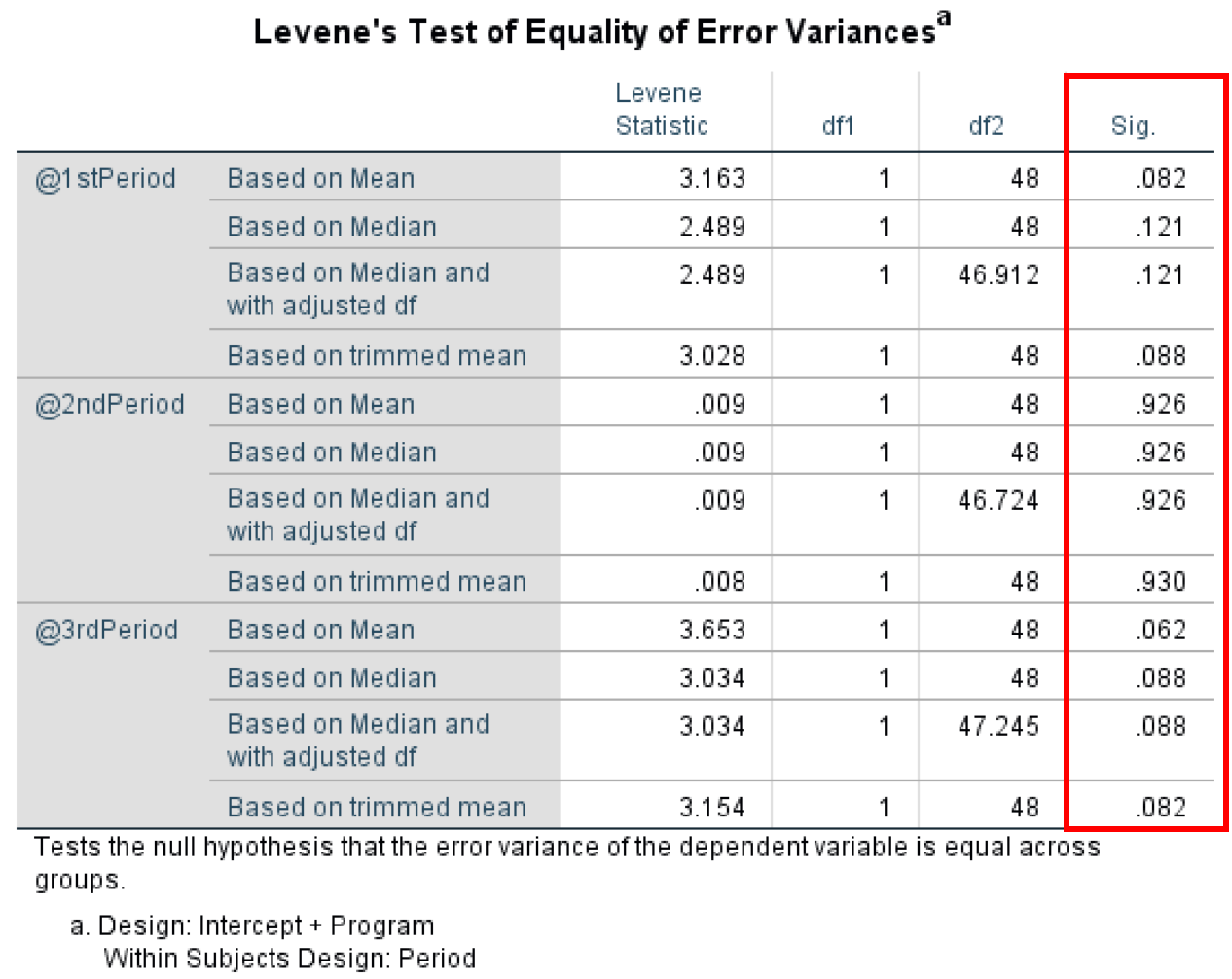
Figure 19: Levene's Test confirming homogeneity of variance assumption is met
- The Tests of Between-Subjects Effects investigates the differences between respondents. The Tests of Between-Subjects Effects have an α level of 0.05. Here we are looking at the effect of the Program variable which shows no statistical significance at P-value = 0.253 as only 0.027 (Partial Eta Squared) of the variance in the dependent variable can be explained by the Program variable.
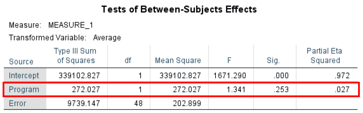
Figure 20: Between-Subjects Effects testing the Program main effect
- The Estimated Margin Means table shows us an estimate summary for the mean and standard error for each period as well as the lower and upper bound values at a 95% confidence interval. You can observe that the Mean in the Estimates table is actually the equivalent of the Total Mean in the Descriptive Statistics table (3).
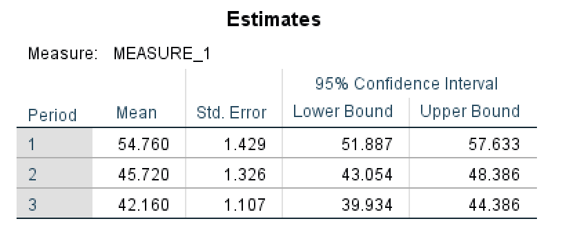
Figure 21: Estimated marginal means for each measurement period
- The Pairwise Comparisontest determines if there are any statistical differences between the pairs – in our case the three Periods of the study. You can see that we have statistical significance between each pair (P-value < 0.05).
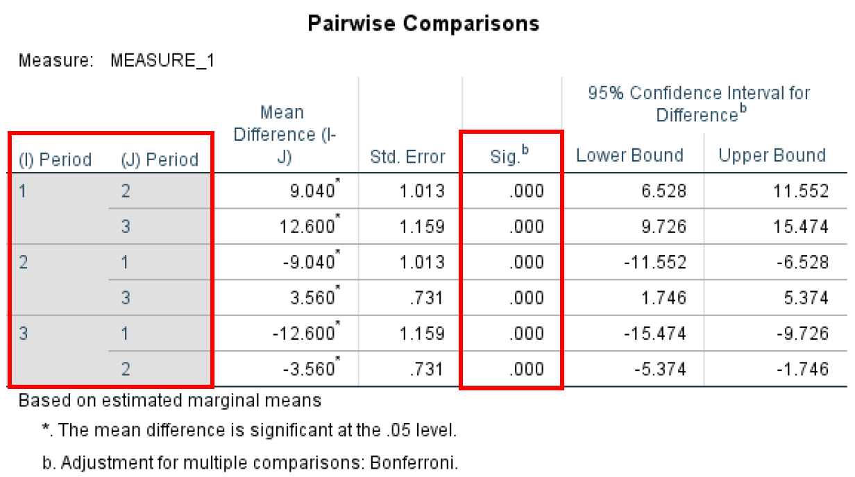
Figure 22: Bonferroni-corrected pairwise comparisons between all time periods
- Finally, the Multivariate Test table shows us a similar output as the Multivariate Test we discussed earlier (5) and shows statistical significance for all the different test statistics used in the ANOVA for repeated measures analysis.
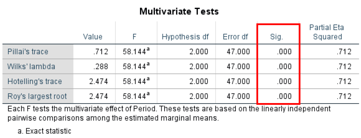
Figure 23: Multivariate test statistics confirming significant differences across time periods
Repeated Measures ANOVA vs One-Way ANOVA
Many researchers confuse repeated measures ANOVA with one-way ANOVA. While both are types of ANOVA, they serve different research designs:
One-Way ANOVA (Between-Subjects):
- Different participants in each group
- Each participant measured once
- Example: Comparing test scores across 3 different teaching methods with 3 separate groups of students
- Assumes independence between groups
One-Way Repeated Measures ANOVA (Within-Subjects):
- Same participants measured multiple times
- Each participant provides data for all conditions/time points
- Example: Measuring the same participants' weight at 3 different time points (baseline, month 1, month 3)
- More statistical power (controls for individual differences)
- Requires sphericity assumption
When to Use Which:
- Use one-way ANOVA when you have independent groups and each participant belongs to only one group
- Use repeated measures ANOVA when you measure the same participants multiple times or under different conditions
- Repeated measures ANOVA is more powerful because it accounts for individual variability
How to Report Repeated Measures ANOVA Results
When reporting your repeated measures ANOVA results in academic writing, include these key elements:
APA Format Example:
"A one-way repeated measures ANOVA was conducted to compare scores on weight loss across three time periods: baseline, 30 days, and 90 days. Mauchly's test indicated that the assumption of sphericity had been violated, χ²(2) = 7.89, p = .02, therefore degrees of freedom were corrected using Greenhouse-Geisser estimates of sphericity (ε = 0.78).
The results show that time had a significant effect on weight loss, F(1.56, 74.88) = 42.35, p < .001, partial η² = .47. Post hoc tests using the Bonferroni correction revealed that weight loss was significantly different between all three time periods (all p values < .05)."
Essential Components to Report:
- Test Used: State you conducted a one-way repeated measures ANOVA
- Variables: Clearly identify your within-subjects factor and levels
- Sphericity: Report Mauchly's test results and any corrections applied (Greenhouse-Geisser or Huynh-Feldt)
- Main Effect: Report F-statistic, degrees of freedom, p-value, and effect size (partial η²)
- Post Hoc Tests: If significant, report which pairs differed (with correction method used)
- Descriptive Statistics: Include means and standard deviations for each time point/condition
Effect Size Interpretation (Partial η²):
- 0.01 = small effect
- 0.06 = medium effect
- 0.14 = large effect
Frequently Asked Questions
Wrapping Up
Here are the key points to remember about repeated measures ANOVA in SPSS:
-
ANOVA for repeated measures is useful when looking to compare the mean scores between three or more groups on different observations. For comparing the means between two groups, the sample T-Test is sufficient.
-
One-way repeated measures ANOVA test is used when a repeated measure design study consists of one independent variable while with the two-way repeated measures ANOVA we use two predictors.
-
To be able to conduct the repeated measures ANOVA test, the study repeated measure design should consist of at least one categorical independent variable and one continuous dependent variable.
References
Cohen, J. (1988). Statistical power for the behavioral sciences (2nd edition). Lawrence Earlbaum: Hillsdale, NJ.
Field, A. (2018). Discovering statistics using IBM SPSS statistics (5th edition). Sage: Thousand Oaks, CA.
Pallant, J. (2010). SPSS survival manual: A step-by-step guide to data analysis using SPSS. Maidenhead: Open University Press/McGraw-Hill.
Pituch, K.A. and Stevens, J.P. (2016) Applied Multivariate Statistics for the Social Sciences.