What is a Measure of Central Tendency?

A measure of central tendency is a fundamental statistical concept that helps you understand the typical or central value in a dataset. In this guide, you'll learn the three main measures (mean, median, and mode), how to calculate each one, and when to use them in your statistical analysis.

Lesson Outcomes

By the end of this article, you should be able to:

Understand the concept of measures of central tendency and their importance in statistics and data analysis.
Define and differentiate between mean, median, and mode as measures of central tendency.
Explain the formulas and procedures to calculate the mean, median, and mode.
Recognize the differences in sensitivity to outliers and applicability among mean, median, and mode.
Interpret histograms and identify the positions of mean, median, and mode in the data distribution.

What is a Measure of Central Tendency?

A measure of central tendency is a single value that represents the center or typical value of a dataset. It provides a way to summarize multiple data points with one representative number. Measures of central tendency help us understand the general behavior or trend of a dataset, making it easier to draw conclusions and make informed decisions based on the data.

There are three main measures of central tendency: the mean, the median, and the mode. Let's explore each of these in more detail.

1. Mean: The Arithmetic Average

The mean, often called the average, is the most common measure of central tendency. It is calculated by adding all the data points in a dataset and dividing by the total number of data points. Here is the mean formula:

\bar{x} = \frac{1}{n} \sum_{i=1}^{n} x_i

Where:

x̄: This symbol represents the mean (average) of the dataset.
n: This represents the total number of data points in the dataset.
xᵢ: This represents each individual data point in the dataset, where i is the index ranging from 1 to n.
Σ (from i=1 to n): This is the summation symbol, which indicates that we should sum the values of xᵢ for all indices from 1 to n. In other words, add up all the data points in the dataset.

When we are looking for a graphical representation of the mean, we should obtain something like the histogram below. Here, we generate a dataset of 100 random numbers with a mean of 50 and a standard deviation of 10.

Histogram with Mean

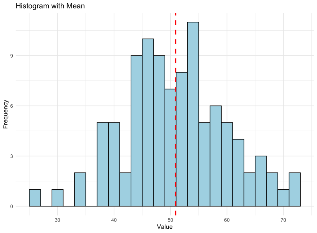
Histogram showing data distribution with the red vertical line representing the mean

NOTE:

A histogram is a visual representation of the dataset. It divides the data into a certain number of bins (groups), and the height of each bar in the histogram represents the frequency (how many times) the data points fall into that specific bin. In other words, taller bars indicate more data points in that range of values.
The vertical red-dotted line in the graphic above represents the mean value of the dataset. The mean is calculated by adding all the data points and dividing the sum by the total number of data points. It provides an idea of the central tendency or "average" of the data.

When you look at the graphic, you can see how the data is distributed, and the vertical line helps you identify where the mean value lies within that distribution. This can give you a general sense of the overall trend in the data and help you understand the dataset's behavior better.

However, it's important to remember that the mean can be sensitive to outliers (extreme values), which might skew the mean and make it less representative of the dataset's central tendency.

Learn how to calculate the mean by hand, Excel, and R in just a few simple steps.

2. Median: The Middle Value

The median is the middle value in a dataset when the data points are arranged in ascending or descending order. While often overlooked, the median is an important measure of central tendency, particularly for skewed distributions.

To find the median, first sort the dataset in ascending or descending order. If there's an odd number of data points, the median is the middle value. If there's an even number of data points, the median is the average of the two middle values. Here's a quick example:

Dataset: $2, 4, 6, 8, 10$ . The median is 6 because it's the middle value.
Dataset: $2, 4, 6, 8$ . The median is 5 because the average is 4 and 6, the two middle values.

One great thing about the median is that it's less sensitive to extreme values, which means it can better represent the center for skewed distributions.

Here is how the graphical representation of a median looks like using the same dataset criteria we used earlier:

Histogram with Median

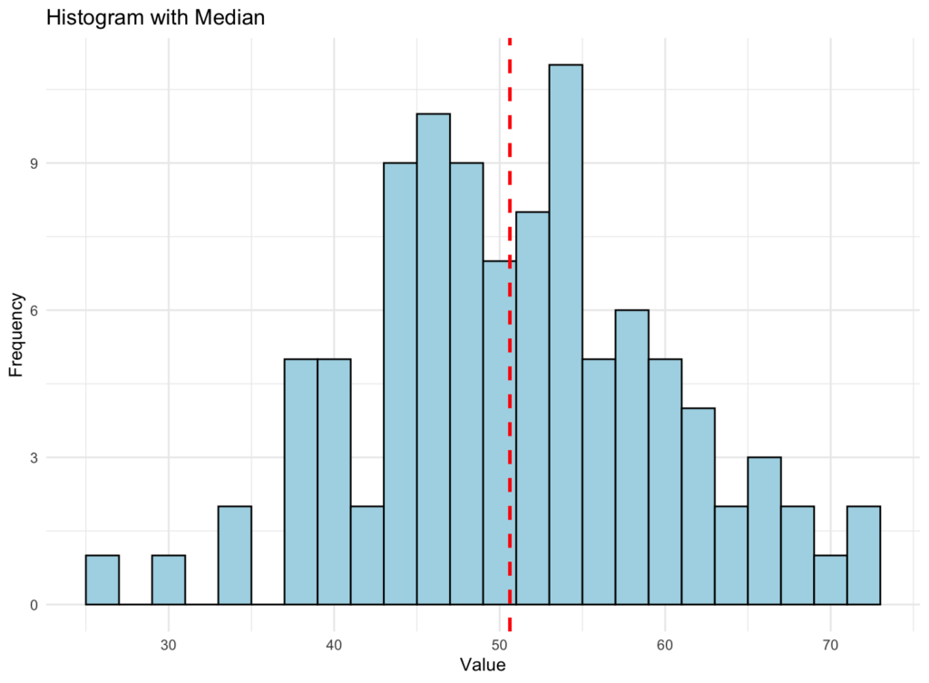
Histogram showing data distribution with the red vertical line representing the median

The median histogram above may look similar to the previous one we generated for the mean. Still, if you pay attention, the red-dotted line representing the median is slightly off. Here is the explanation why:

The mean (average) is calculated by adding up all the data points and dividing the sum by the total number of data points. It gives an idea of the central tendency or "average" of the data. However, the mean can be sensitive to outliers (extreme values) and may not represent the true center of the dataset when outliers are present.
The median is the middle value of the dataset represented by the red-dotted line when the data is sorted in ascending or descending order. If there is an even number of data points, the median is the average of the two middle values. The median is less sensitive to outliers than the mean and can better represent the dataset's central tendency when outliers are present.

NOTE: In the generated histograms, the vertical lines for the mean and median are slightly different because they represent different measures of central tendency. Their positions may vary depending on the dataset's distribution of data points. In some cases, the mean and median may be close or equal. In contrast, in other cases, they may be different due to the presence of outliers or the specific distribution of the data.

Learn how to calculate the median by hand, Excel, and R easily.

3. Mode: The Most Frequent Value

The mode is the value that occurs most frequently in a dataset. It represents the most common observation in your data.

Unlike the mean, there isn't a specific mathematical equation to calculate the mode. The mode is simply the value or values that occur most frequently in a dataset. To find the mode, you need to count the frequency of each unique value in the dataset and identify the one(s) with the highest frequency.

In some cases, a dataset might have:

One mode (unimodal): A single value occurs more frequently than any other value.
Two modes (bimodal): Two different values occur with the same highest frequency.
Multiple modes (multimodal): More than two values occur with the same highest frequency.
No mode: All values in the dataset occur with the same frequency.

It's important to note that the mode can be used for any type of data, including nominal, ordinal, interval, or ratio data, as it only relies on the frequency of each unique value.

The histogram for the mode, along with a vertical line representing the mode value, looks like this:

Histogram with Mode

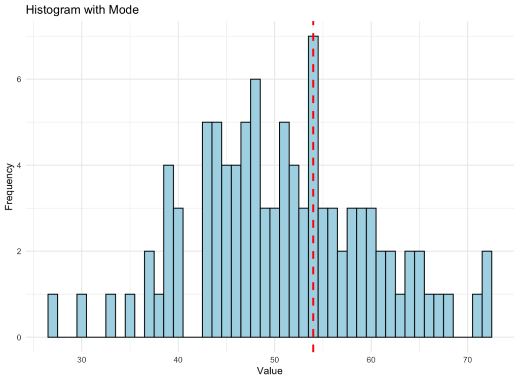
Histogram showing data distribution with the red vertical line representing the mode

Here is a simple breakdown of what the mode histogram above tells us:

The histogram is a visual representation of the dataset. It divides the data into a certain number of bins (groups), and the height of each bar in the histogram represents the frequency (how many times) the data points fall into that specific bin. In other words, taller bars indicate more data points in that range of values.
The vertical red-dotted line in the graphic represents the mode value of the dataset. The mode is the value that occurs most frequently in the dataset. It is a measure of central tendency that can help identify the dataset's most common value or values.

When looking at the mode histogram, you can see how the data is distributed, and the vertical line helps you identify where the mode value(s) lie within that distribution.

The mode can provide insights into the dataset's general behavior and help you understand the most common values. Unlike the mean and median, the mode is unaffected by outliers or extreme values, making it a suitable measure of central tendency when the dataset has a skewed distribution or contains outliers.

Learn how to calculate the mode by hand, Excel, and R quickly.

Why Do We Care About Measures of Central Tendency?

Measures of central tendency are used to analyze and interpret data in various fields, such as statistics, economics, psychology, and other sciences. They help us to:

Summarize large datasets: Instead of analyzing every single data point, we can use a measure of central tendency to get a general idea of what the data looks like. This simplifies our analysis and makes understanding the overall pattern or trend in the data easier.
Compare different datasets: Measures of central tendency allow us to compare datasets by providing a single value representing each dataset's center. This makes it easier to see which dataset has higher or lower values on average.
Identify trends and patterns: By looking at the mean, median, or mode, we can identify trends and patterns in the data. This can be useful for making predictions, identifying areas for improvement, or monitoring changes over time.
Make informed decisions: In many fields, decision-makers rely on measures of central tendency to guide their choices. For example, a business owner might look at the average revenue of different products to decide which ones to focus on promoting, or a teacher might use the median test score to determine the effectiveness of their teaching methods.

How To Choose The Right Measure of Central Tendency

Now that you know what a measure of central tendency is and why it's important, you might be wondering which one to use in different situations. Here are some general guidelines to help you choose the right measure for your needs:

Use the mean when: Your data is relatively symmetric and free of extreme values or outliers. The mean is great for providing an overall trend in the data and is commonly used in many fields.
Use the median when: Your data is skewed or has extreme values that might affect the mean. The median is less sensitive to outliers and better represents the center for skewed distributions.
Use the mode when: You want to identify a dataset's most frequent or popular value. The mode is particularly useful for categorical or discrete data where other measures of central tendency might not be applicable.

Frequently Asked Questions

What is the difference between mean, median, and mode?

Mean is the arithmetic average calculated by summing all values and dividing by the count. Median is the middle value when data is ordered from smallest to largest. Mode is the most frequently occurring value in a dataset. Each measure serves different purposes: mean is best for normally distributed data without outliers, median works well with skewed data or outliers, and mode is ideal for categorical data or finding the most common value.

When should I use the median instead of the mean?

Use the median instead of the mean when your data contains outliers or is skewed (not normally distributed). The median is resistant to extreme values because it only considers the middle position, not the actual values. For example, in income data where a few very high earners can skew the mean upward, the median provides a more representative measure of the typical income. The median is also preferred when working with ordinal data or when extreme values don't represent the central tendency accurately.

Can a dataset have more than one mode?

Yes, a dataset can have multiple modes. When a dataset has two modes, it's called bimodal; with three modes, it's trimodal; and with more than three, it's multimodal. For example, in a dataset of test scores (65, 70, 70, 80, 85, 85, 90), both 70 and 85 are modes because they appear twice. A dataset with no repeating values has no mode. Multiple modes can indicate different subgroups within your data or multiple peaks in the distribution.

How do outliers affect measures of central tendency?

Outliers significantly affect the mean because it uses all values in its calculation - a single extreme value can pull the mean away from the typical center. The median is resistant to outliers because it only considers the middle position, not the actual extreme values. The mode is completely unaffected by outliers unless the outlier itself is the most frequent value. For example, in the dataset (10, 12, 13, 14, 100), the mean is 29.8 (heavily influenced by 100), but the median remains 13 (representative of the typical value).

What does it mean when mean, median, and mode are equal?

When mean, median, and mode are equal (or very close), it indicates a symmetric, normal distribution with no skewness. This is the classic bell-shaped curve where data is evenly distributed around the center. In such distributions, all three measures point to the same central value, making any of them a reliable measure of central tendency. This is common in naturally occurring phenomena like human height, test scores in large populations, or measurement errors.

How do I calculate the median with an even number of values?

When you have an even number of values, the median is the average of the two middle values. First, arrange your data in order from smallest to largest. Then identify the two middle numbers and calculate their average. For example, in the dataset (3, 5, 7, 9), the two middle values are 5 and 7. The median is (5 + 7) / 2 = 6. With an odd number of values, the median is simply the middle value after ordering the data.

Which measure of central tendency is best for categorical data?

Mode is the only appropriate measure of central tendency for categorical (nominal) data because you cannot calculate a meaningful average or middle value for categories like colors, names, or types. For example, if you survey favorite colors and get (red, blue, blue, green, blue, red, blue), the mode is blue (appears 4 times). You cannot calculate a mean or median for color categories because they don't have numerical values or a natural ordering. For ordinal data (ordered categories like rankings), you can use mode or median, but not mean.

What is a weighted mean and when is it used?

A weighted mean assigns different levels of importance (weights) to different values in your dataset, rather than treating all values equally. It's calculated by multiplying each value by its weight, summing these products, and dividing by the sum of weights. The formula is: Weighted Mean = Σ(value × weight) / Σ(weights). Use weighted means when some observations are more important than others, such as calculating grade point averages (where different courses have different credit hours), financial indices (where companies have different market capitalizations), or survey data (where responses are weighted to match population demographics).

Wrapping Up

Measures of central tendency (mean, median, and mode) provide essential tools for summarizing and understanding data distributions. Each measure offers unique advantages. The mean provides an overall average, the median resists the influence of outliers, and the mode identifies the most common value in your dataset.

By selecting the appropriate measure of central tendency for your specific data characteristics and research questions, you can draw more accurate conclusions and make better-informed decisions from your statistical analyses.