Multiple linear regression is one of the most powerful statistical techniques for analyzing the relationship between multiple independent variables and a single dependent variable. In this comprehensive guide, you'll learn how to run multiple regression in SPSS, interpret multiple regression output in SPSS, and understand every component of the analysis results.
Whether you're investigating marketing effectiveness, predicting academic performance, or analyzing any relationship with multiple predictors, this tutorial covers everything from data preparation to results interpretation. I'll provide you with a complete SPSS dataset for multiple linear regression analysis so you can follow along step-by-step.
Multiple regression analysis in SPSS is straightforward. If you know how to calculate a simple linear regression in SPSS, you'll find the process nearly identical. The main difference is interpreting results with multiple predictors, and we'll cover every parameter in detail.
What is Multiple Linear Regression Explained with Example
With simple linear regression, we analyze the causal relationship between a single independent variable and a dependent variable. In other words, we aim to see if the independent variable (predictor) has a significant effect on the dependent variable (outcome). But how do we analyze regression when a model contains multiple independent variables?
Say hello to multiple linear regression analysis.
In multiple linear regression analysis, we test the effect of two or more predictors on the outcome variable, hence the term multiple linear regression.
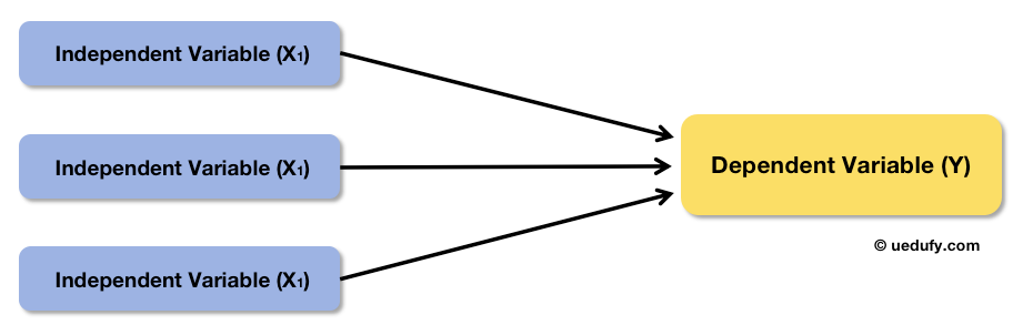
Figure 1: Multiple linear regression analyzes the relationship between multiple predictors and one outcome
In terms of analysis, for both simple and multiple linear regression the goal remains pretty much the same: finding if there is any significance (P-value) between the multiple predictors and outcome. If the P-value is equal to or lower than 0.05 (P ≤ 0.05) the predictor-outcome relationship is significant.
Let's look at an example of multiple linear regression. Suppose we want to investigate the relationship between marketing efforts and consumer purchase intention of a company. In this case, the predictor variable is marketing efforts and the outcome is purchase intention.
I know what you're thinking. "Marketing efforts" is such a broad term and so many factors can contribute to it. There's no point investigating marketing efforts as a whole if we can't identify which factors are more important than others, right?
Let's split marketing efforts into several independent variables (X), e.g., content marketing (X1), social media marketing (X2), and email marketing (X3). Here is what the conceptual framework for this example looks like:
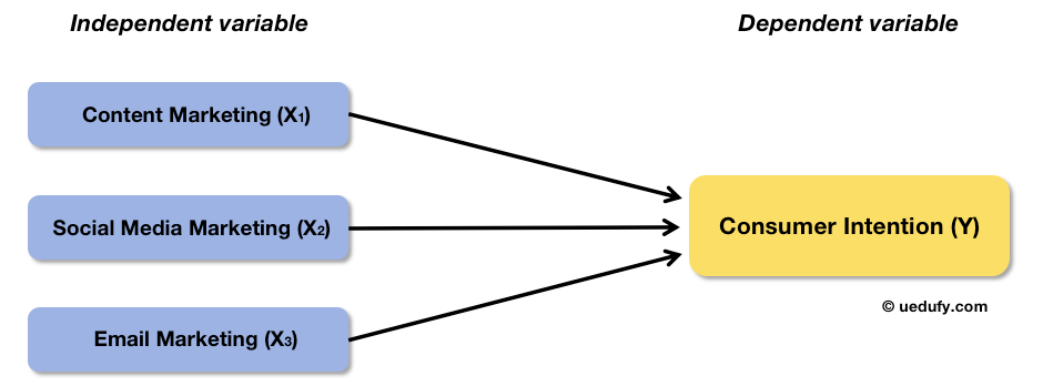
Figure 2: Example conceptual framework with marketing efforts broken into three predictors
Now that we got our conceptual framework, let's jump into action and do multiple regression analysis in SPSS using the example we discussed above.
Calculate Multiple Linear Regression using SPSS
Calculating multiple linear regression using SPSS is very much the same as doing a simple linear regression analysis in SPSS. If you want to follow along, download the SPSS dataset from the Download section in the sidebar.
The example SPSS data set contains 30 samples where the Content, SocialMedia, Email are independent variables (predictors), and Consumer_Intention is the dependent variable (outcome). After downloading, unzip the file and double-click on the file with the .sav extension to import the data set in SPSS.
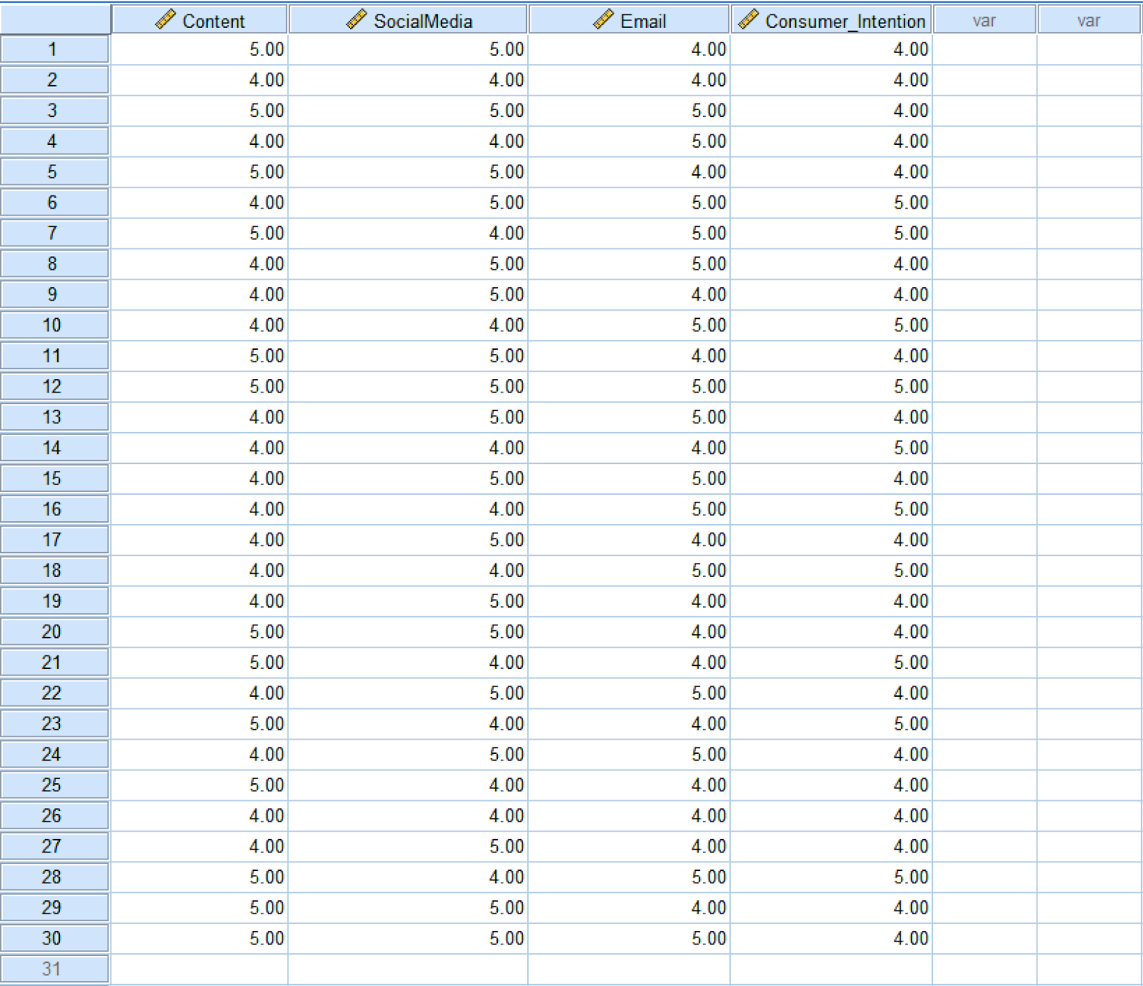
Figure 3: Example dataset with three predictors and one outcome variable
Next, let's learn how to calculate multiple linear regression using SPSS for this example.
- In SPSS top menu, go to Analyze → Regression → Linear.
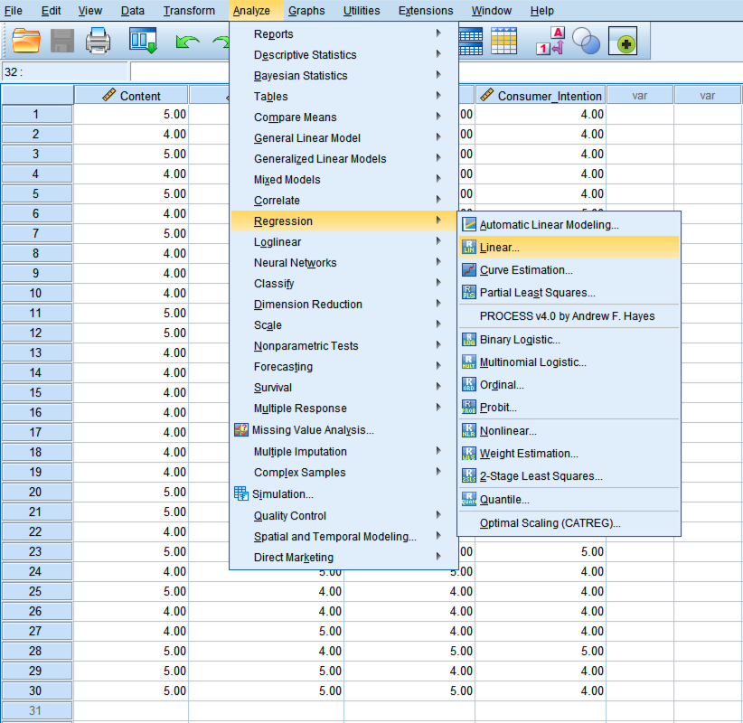
Figure 4: Navigate to Analyze, Regression, Linear in SPSS
- On the Linear Regression window, use the arrow button to move the outcome Consumer_Intention to the Dependent box. Do the same with the predictor variables Email, Content, and SocialMedia to move them to the Independent(s) box.
Make sure the linear regression method is set to Enter.
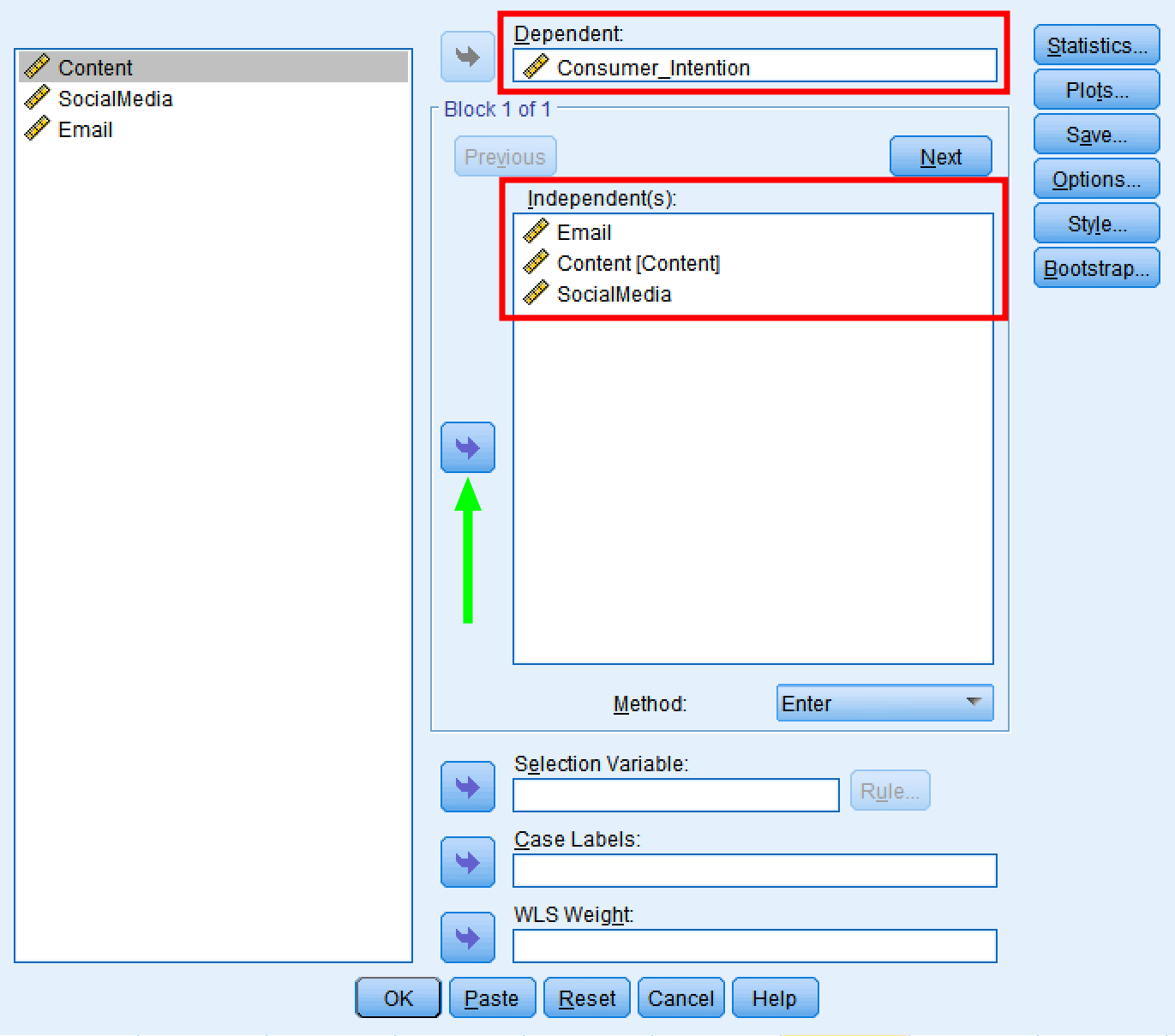
Figure 5: Select dependent and independent variables in Linear Regression dialog
- Click the OK button to calculate multiple linear regression using SPSS. A new window containing the multiple linear regression results will appear.
Interpret Multiple Linear Regression Output in SPSS
Now we got our multiple linear regression results in SPSS, let's look at how to interpret the output. By default, SPSS will show four tables in the regression output:
- Variables Entered/Removed
- Model Summary
- ANOVA
- Coefficients
Let's have a look at each table and understand what those terms and values mean.
Variables Entered/Removed
This table contains an analysis summary of the multiple linear regression using SPSS respectively the regression model used, the independent and dependent variables entered in analysis, as well as the regression method.
In some cases, SPSS will choose to remove variables from the model if they are found to cause multicollinearity issues. In this regression analysis, no variables were removed therefore we can deduce that no variables were found to be linearly dependent on one another.
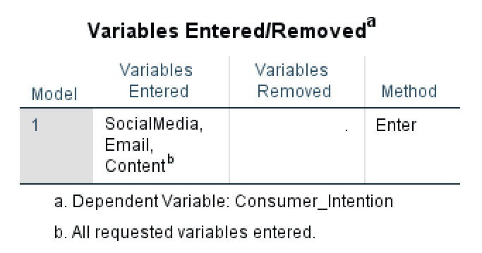
Figure 6: Variables Entered/Removed table showing all predictors included in the model
Model Summary
The Model Summary table provides key statistics about how well the regression model fits the data. This table includes three critical measures: R, R², and Adjusted R².
R (Multiple Correlation Coefficient) represents the correlation between the observed values and the predicted values of the dependent variable. It ranges from 0 to 1, with higher values indicating better prediction. In our example, R indicates the strength of the relationship between all three predictors combined and Consumer_Intention.
R² (Coefficient of Determination) tells us the proportion of variance in the dependent variable that is explained by the independent variables. It's calculated as:
In our case:
This means our three predictors (Email, Content, SocialMedia) explain 44.3% of the variation in Consumer_Intention. The remaining 55.7% is unexplained variance.
Adjusted R² modifies R² to account for the number of predictors in the model. It's more accurate for comparing models with different numbers of predictors because it penalizes adding unnecessary variables. The formula is:
Where:
- n = sample size (30 in our case)
- k = number of predictors (3 in our case)
Adjusted R² will always be slightly lower than R², especially with smaller sample sizes or more predictors. When comparing models, prefer the one with higher Adjusted R².
ANOVA
The ANOVA table in multiple regression tests whether the regression model as a whole significantly explains variance in the dependent variable. It compares the variance explained by the model (Regression) against the unexplained variance (Residual). If the model explains significantly more variance than error, the F-test will be significant.
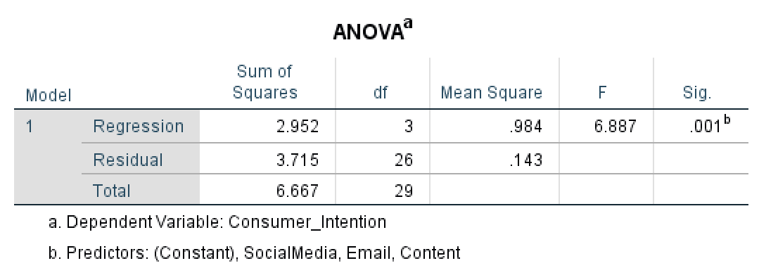
Figure 7: ANOVA table displaying regression model fit statistics
Let's start with the Sum of Squares column in ANOVA. The Regression Sum of Squares (SSR) shows the amount of variation in the dependent variable explained by the independent variables. In our case, the regression model explains 2.952 units of variation. Higher Regression SS values indicate the model explains more variance in the outcome - which is desirable.
The Residual Sum of Squares (SSE) measures the unexplained variation or error in the model. In our case, the Residual Sum of Squares is 3.715. Lower residual values are better, as they indicate less unexplained variance. A residual of zero would mean perfect prediction.
The Total Sum of Squares is calculated by adding the Regression Sum of Squares and Residual Sum of Squares respectively 6.667 in our case.
Next, let's look at the Degree of Freedom (df) column in ANOVA.
The Regression df equals the number of predictor variables in the model (k). In our case, we have 3 predictors (Email, Content, SocialMedia), so regression df = 3.
The Residual df is calculated as: n - k - 1, where n is the sample size, k is the number of predictors, and 1 accounts for the intercept. With 30 samples and 3 predictors:
The Total df equals n - 1 (sample size minus one), which is 29 in our example.
The Regression Mean Square is calculated by dividing the regression sum of squares divided by the regression degree of freedom – in our example 0.984. The Residual Mean Square is computed in the same way, by dividing the residual sum of squares by the residual degree of freedom – respectively, 0.143 in our case.
The F column in ANOVA represents the F statistics which is probably the most important quantity in the ANOVA test. The F statistics equals the ratio between Regression Mean Square and Residual Mean Square and is used to calculate the P-value. In our example, the F statistics equals 6.887.
Finally, the Sig. column in ANOVA (P-value) tells us if the difference between the groups in the regression model is significant. Since in our case the P is 0.001 respectively ≤ 0.05, the difference between Content, SocialMedia, and Email groups are statistically significant.
Coefficients
The last table in the regression output is the Coefficients table. Here we can find details about the Unstandardized Coefficient Beta and Standard Error, Standardized Coefficient Beta, the t and P-value the predictors in our model.
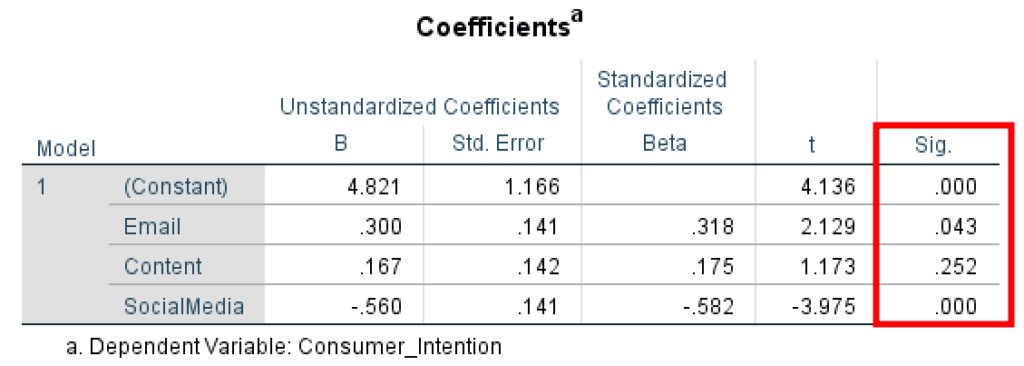
Figure 8: Coefficients table showing the statistical significance of each predictor
The Unstandardized Coefficient Beta measures the variation in the outcome variable for one unit of change in the predictor variable, where the raw values are displayed in the original scale.
The Standard Error of the estimates measures the average distance of the observed data points from the regression line. A large standard error value indicates that sample means are distributed widely around the population mean. A low standard error value indicates that the mean of the sample and the mean of the population are closely correlated – a good thing.
The Standardized Coefficients Beta (also known as beta weights) measures the effect of each predictor when all variables are standardized to have a mean of 0 and standard deviation of 1. This allows you to compare the relative importance of predictors measured on different scales. A larger absolute standardized beta indicates a stronger effect.
The t statistics column shows the measure of the standard deviation of the coefficient and is calculated by dividing the Beta coefficient by its standard error. In general, a value larger than +2 or -2 is considered acceptable.
Finally, the Sig. (P-value) column in the regression coefficients shows the statistical significance for each predictor on the outcome variable where a P-value ≤ 0.05 is considered acceptable.
In our example, we can observe that the predictor variable Email has an effect on the outcome variable Consumer_Intention (P = 0.043, < 0.05) therefore the relationship is statistically significant.
The predictor Content has no effect on the outcome Consumer_Intention (P = 0.252, > 0.05) therefore no statistical significance in the regression model.
The predictor SocialMedia has an effect on the Consumer_Intention (P = 0.000, < 0.05) therefore the relationship between the two variables is statistically significant.
In conclusion, the most important values you should check when looking to interpret multiple linear regression output in SPSS are:
- One-way ANOVA test results tell us if the difference between the groups in the regression model is significant at P ≤ 0.05.
- Regression coefficient showing a significant effect between predictor and outcome variable at P ≤ 0.05.
Export Linear Regression Output in SPSS
Finally, let's export the multiple linear regression using SPSS results as a .pdf file for further use. On the regression results Output window, click on File → Export.
- In the Export Output window, select the Portable Document Format (*.pdf) option. Other options such as Word/RTF (.doc) and PowerPoint (.ppt) export options are available in case you prefer those formats.
- Type a File Name and Browse for the location you prefer to save your multiple linear regression results in SPSS.
- Click the OK button to export the SPSS output.
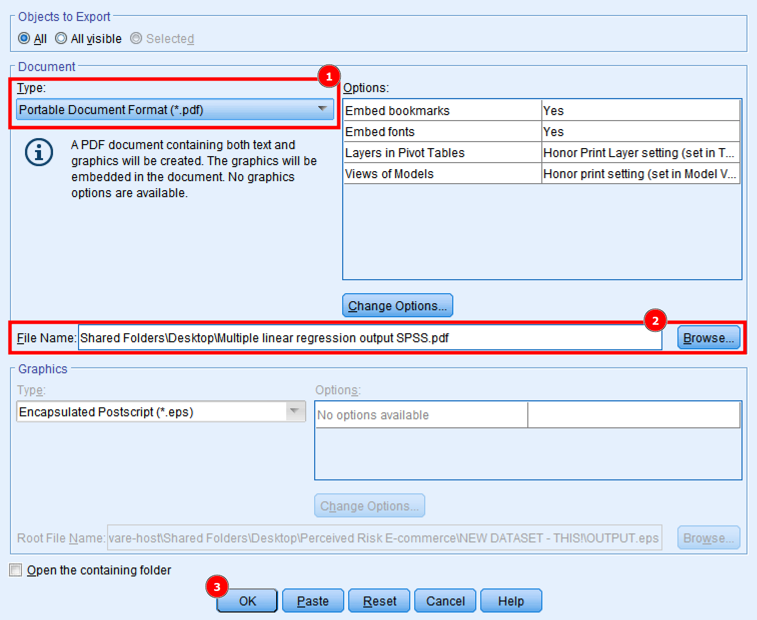
Figure 9: Export regression output to PDF, Word, or PowerPoint format
The file containing the multiple linear regression output in SPSS is now available for your further use.
Assumptions of Multiple Linear Regression
Before interpreting your results, it's crucial to verify that your data meets the assumptions of multiple linear regression. Violating these assumptions can lead to inaccurate or misleading results.
1. Linearity
The relationship between each independent variable and the dependent variable should be linear. You can check this by creating scatterplots of each predictor against the outcome variable.
How to test in SPSS: Create scatterplots (Graphs → Legacy Dialogs → Scatter/Dot) for each predictor-outcome pair. Look for a linear pattern rather than curved relationships.
2. Independence of Observations
Observations should be independent of each other. This assumption is violated in cases like repeated measures, time series data, or clustered data.
How to ensure: Check your research design. If you have repeated measures or clustered data, you'll need more advanced techniques like mixed models or generalized estimating equations.
3. Homoscedasticity
The variance of residuals should be constant across all levels of the independent variables. In other words, the spread of residuals should be roughly equal across the regression line. Learn more about what homoscedasticity means in statistics.
How to test in SPSS: In Linear Regression dialog, click Plots → add ZPRED to X-axis and ZRESID to Y-axis. The resulting scatterplot should show randomly scattered points with no cone or fan pattern.
4. Normality of Residuals
The residuals (errors) should be approximately normally distributed. This is especially important for smaller sample sizes.
How to test in SPSS: In Linear Regression dialog, click Plots → check "Histogram" and "Normal probability plot." The histogram should resemble a bell curve, and points on the P-P plot should fall close to the diagonal line.
5. No Multicollinearity
Independent variables should not be too highly correlated with each other. High multicollinearity inflates standard errors and makes it difficult to assess the individual effect of each predictor.
How to test in SPSS: In Linear Regression dialog, click Statistics → check "Collinearity diagnostics." Look at VIF (Variance Inflation Factor) values. VIF values above 10 indicate problematic multicollinearity. Tolerance values below 0.1 also suggest issues.
6. No Significant Outliers or Influential Cases
Extreme values can disproportionately affect the regression line and lead to misleading results.
How to test in SPSS: In Linear Regression dialog, click Save → check "Cook's distance" and "Standardized residuals." Cook's distance values above 1 suggest influential cases. Standardized residuals beyond ±3 indicate potential outliers.
Frequently Asked Questions
Wrapping Up
I hope by now you got an understanding of how to calculate multiple linear regression using SPSS as well as how to interpret multiple linear regression output in SPSS. As you can see, is not that difficult.
If this is the first time you perform a linear regression in SPSS, I recommend you to repeat the process a few times more as well as try using your dataset for multiple linear regression analysis.