The paired samples t-test compares two measurements taken from the same participants. It is the standard analysis for pre-test/post-test designs, before-and-after studies, and any research where the same group is measured twice under different conditions. Unlike the independent samples t-test, which compares two separate groups, the paired test accounts for the within-subject correlation between measurements, giving it more statistical power to detect a real difference.
This guide walks through the full process in SPSS: checking assumptions, running the test, interpreting all three output tables, calculating Cohen's d for paired designs, and reporting results in APA 7th format. If you followed the independent samples t-test guide, note that the paired version has different normality requirements and a different effect size formula. The tutorial uses an extended version of the thesis dataset from previous guides, with two new variables added for pre-test and post-test scores.
Key Takeaways:
- The paired samples t-test compares two measurements from the same participants (e.g., pre-test vs. post-test, before vs. after intervention)
- The normality assumption applies to the difference scores, not to each variable individually
- SPSS computes the difference as Variable 1 minus Variable 2, which often produces a negative t-value when scores improve. This is not an error.
- Cohen's d for paired designs uses a different formula than the independent version: d = Mean of Differences / SD of Differences
- Report the t statistic, degrees of freedom, p-value, both means with SDs, and effect size in your Results chapter
Before you begin: This guide assumes you have your data loaded in SPSS with two related measurements (e.g., pre-test and post-test scores) defined in Variable View. You should have already examined descriptive statistics for your variables. If you need to check normality of the difference scores, see our guide on how to check normality in SPSS.
When to Use a Paired Samples T-Test
The paired samples t-test is appropriate when your research design meets these conditions:
- You have one continuous dependent variable measured at two time points or under two conditions.
- The same participants provide both measurements (or participants are matched in pairs).
- You want to determine whether the mean difference between the two measurements is statistically significant.
If the two measurements come from different participants, use the independent samples t-test instead. If you have three or more related measurements, use repeated measures ANOVA.
Common thesis examples:
| Research Question | Variable 1 | Variable 2 | Design |
|---|---|---|---|
| Does the training program improve test scores? | PreTestScore | PostTestScore | Pre/post intervention |
| Do students rate the course differently at midterm vs. final? | MidtermRating | FinalRating | Two time points |
| Is there a difference between self-reported and observed behavior? | SelfReport | ObservedScore | Two measurement methods |
Table 1: Common research designs suitable for the paired samples t-test
Assumptions
The paired samples t-test has three assumptions. Two of them are straightforward; the third requires a specific check that differs from the independent t-test.
1. Related Observations (Paired Data)
Each case in the dataset must have both measurements. Participant 1 has a pre-test score and a post-test score; participant 2 has a pre-test score and a post-test score; and so on. This is met through research design. If some participants dropped out between measurements, SPSS handles this through listwise deletion (those cases are excluded from the analysis).
2. Continuous Dependent Variable
Both measurements must be on an interval or ratio scale. Test scores, ratings on a continuous scale, and physiological measurements all qualify. Ordinal data with few categories (e.g., a 3-point scale) is better analyzed with the Wilcoxon signed-rank test.
3. Normality of the Difference Scores
This is where the paired t-test differs from the independent version. The normality assumption does not apply to each variable separately. It applies to the difference scores (Variable 1 minus Variable 2 for each participant).
To check this:
- Create a new variable: Transform > Compute Variable. Set the target variable to something like
Differenceand the expression toPostTestScore - PreTestScore. - Test normality on this new variable using the Explore procedure, as described in the normality guide.
With 30 or more participants, the paired t-test is robust to moderate normality violations (Schmider et al., 2010). With our sample of 150, this assumption is easily met. If your sample is small and the difference scores are severely non-normal, use the Wilcoxon signed-rank test as the non-parametric alternative.
Note that Levene's test for equality of variances, which is part of the independent t-test workflow, does not apply here. There is only one group, measured twice, so there are no between-group variances to compare.
Example Dataset
This tutorial uses an extended version of the thesis dataset from the descriptive statistics and normality guides. Two new variables have been added to the dataset: PreTestScore and PostTestScore, representing scores before and after a study skills intervention. You can download the extended dataset from the sidebar.
Research question: Did the study skills intervention improve test scores?
- Variable 1: PreTestScore (continuous, Scale, range 40-90)
- Variable 2: PostTestScore (continuous, Scale, range 45-95)
- Sample: 150 participants measured before and after the intervention
- Design: Single-group pre-test/post-test
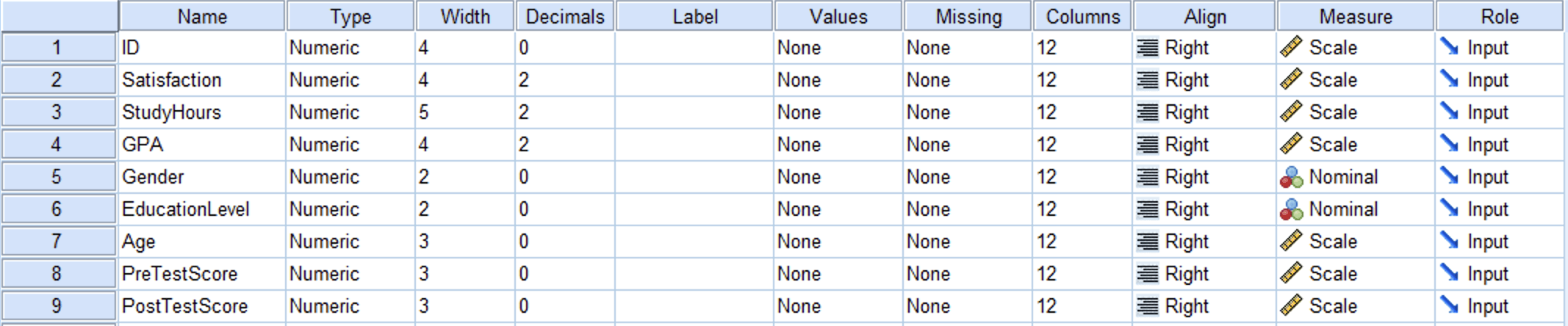
Figure 1: Variable View in SPSS showing the PreTestScore and PostTestScore variables
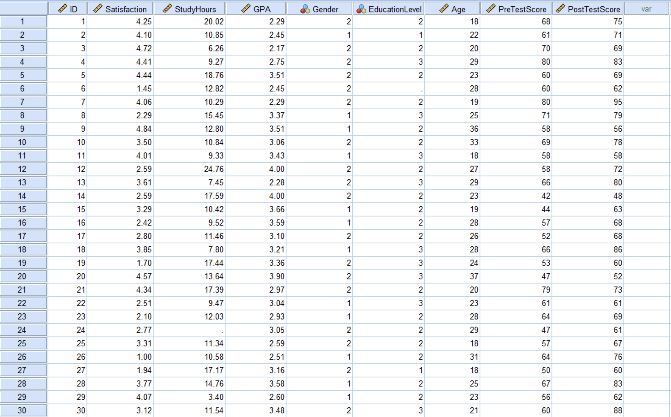
Figure 2: Data View in SPSS with pre-test and post-test scores for 150 participants
Step-by-Step: Running the Paired Samples T-Test
Step 1: Navigate to the T-Test Dialog
Go to Analyze > Compare Means > Paired-Samples T Test.
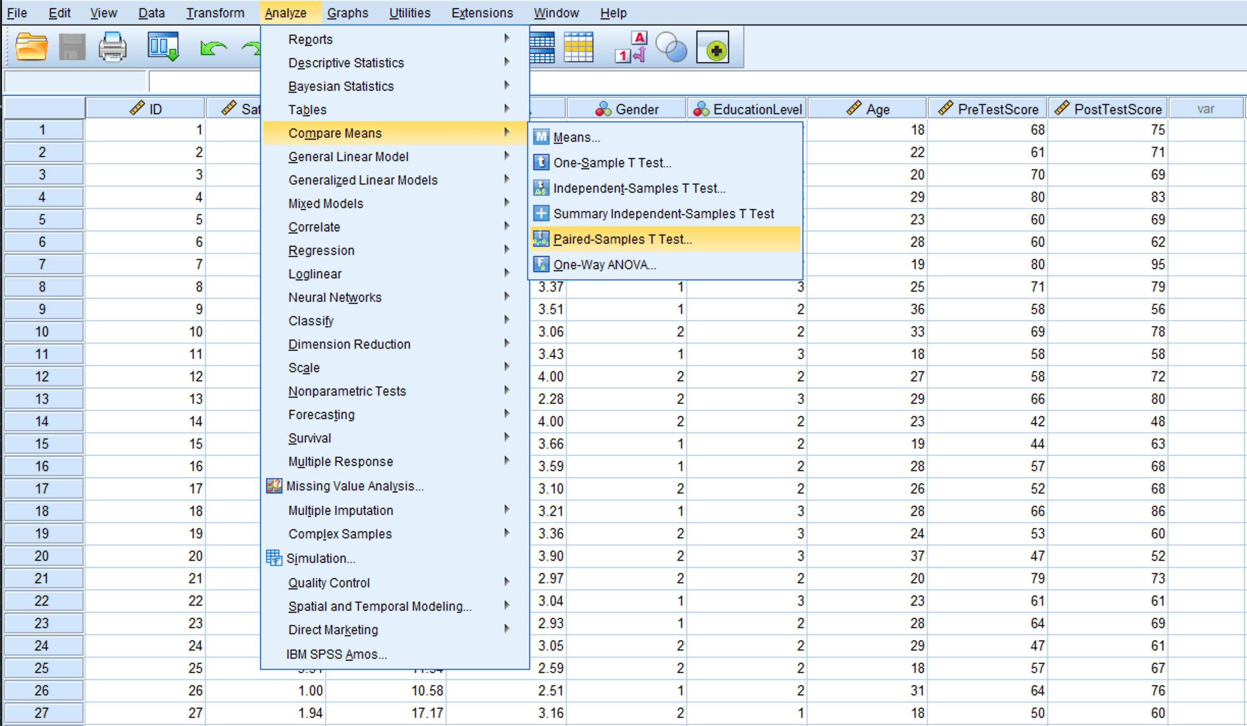
Figure 3: Navigate to Analyze > Compare Means > Paired-Samples T Test
Step 2: Select the Paired Variables
In the Paired-Samples T Test dialog:
- Select PreTestScore from the left variable list.
- Hold Ctrl (or Cmd on Mac) and also select PostTestScore.
- Click the blue arrow button to move both variables into the Paired Variables box.
- SPSS displays them as Pair 1: PreTestScore - PostTestScore.
The order matters for the sign of the output. SPSS calculates Variable 1 minus Variable 2 (PreTestScore minus PostTestScore). Since we expect post-test scores to be higher, the mean difference will be negative. This is not an error.
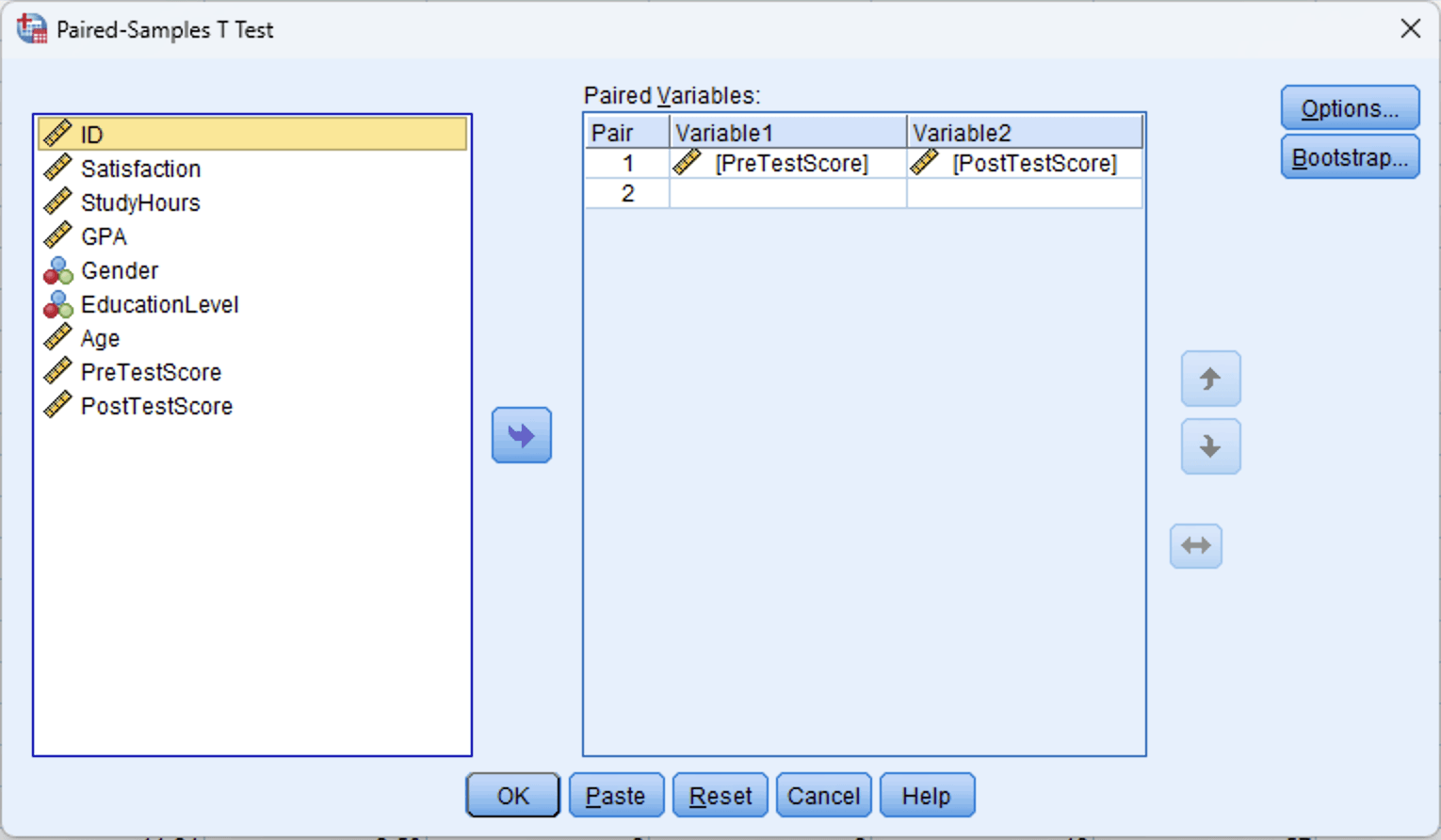
Figure 4: Paired-Samples T Test dialog with PreTestScore as Variable 1 and PostTestScore as Variable 2
Step 3: Run the Test
Click OK. SPSS produces three output tables: Paired Samples Statistics, Paired Samples Correlations, and Paired Samples Test.
Interpreting the Output
SPSS generates three tables for the paired samples t-test. Each provides different information, and you will need values from all three for a complete interpretation and APA report.
Paired Samples Statistics Table
This table reports the descriptive statistics for each variable separately.
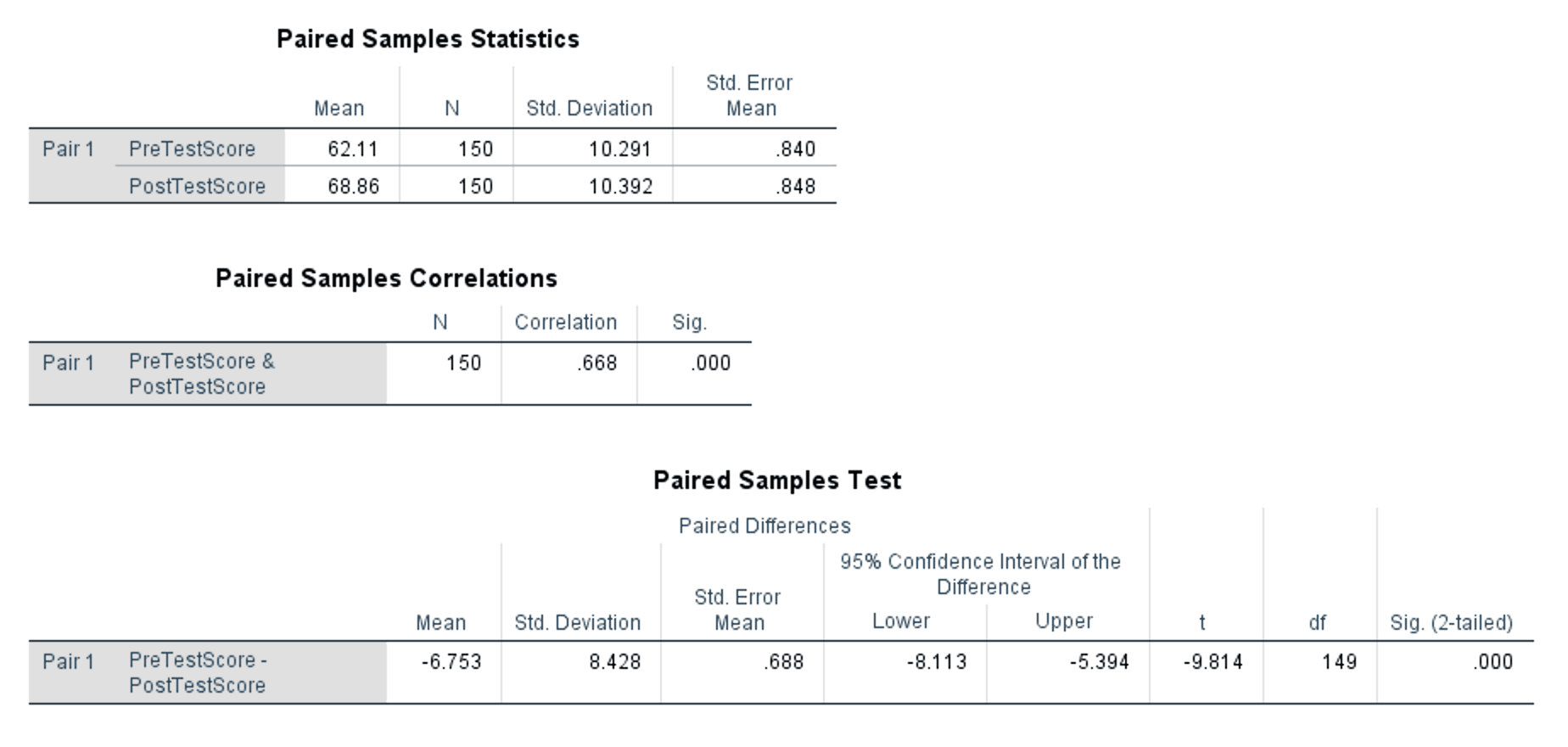
Figure 5: Complete paired samples t-test output showing all three tables
What to look at:
- Mean: PreTestScore = 62.11, PostTestScore = 68.86. Post-test scores are on average 6.75 points higher.
- N: 150 for both variables. No cases were excluded due to missing data.
- Std. Deviation: PreTestScore = 10.291, PostTestScore = 10.392. The spread of scores is similar across both measurements.
- Std. Error Mean: The precision of each mean estimate. Smaller values indicate more precise estimates.
Paired Samples Correlations Table
This table shows the Pearson correlation between the two measurements.
- Correlation: .668, Sig.: .000 (p < .001)
The correlation of .668 is moderate to strong and statistically significant. This confirms that pre-test and post-test scores are positively related: participants who scored higher before the intervention also tended to score higher after it. This is expected in a within-subjects design and is one reason the paired t-test has more power than the independent version. By accounting for this correlation, the paired test removes between-subject variability from the error term.
If this correlation were near zero or negative, it would suggest something unusual about your data (e.g., the pairing structure may be wrong, or the two measurements may not be from the same construct).
Paired Samples Test Table
This is the main results table. It reports the paired differences and the t-test result.
Reading the Paired Differences columns:
- Mean: -6.753. This is the average of all individual differences (PreTestScore minus PostTestScore). The negative sign means post-test scores are higher than pre-test scores on average.
- Std. Deviation: 8.428. This is the standard deviation of the difference scores, not of either variable individually. You will need this value for calculating Cohen's d.
- Std. Error Mean: 0.688. The standard error of the mean difference.
- 95% Confidence Interval: [-8.113, -5.394]. The entire interval is negative, meaning we are 95% confident the true population mean difference falls between -8.11 and -5.39. Because the interval does not contain zero, the difference is statistically significant.
Reading the test statistics:
- t: -9.814. The t statistic is negative because the mean difference is negative (pre-test scores minus post-test scores). The absolute value (9.814) represents how many standard errors the mean difference is from zero.
- df: 149 (N - 1 = 150 - 1).
- Sig. (2-tailed): .000 (p < .001). The result is statistically significant at any conventional alpha level.
Putting the Output Together
The paired samples t-test shows a statistically significant increase in test scores from pre-test (M = 62.11, SD = 10.29) to post-test (M = 68.86, SD = 10.39), with a mean improvement of 6.75 points. The 95% confidence interval for the mean difference [-8.11, -5.39] does not include zero, and the t-test is significant, t(149) = -9.81, p < .001.
The correlation between pre-test and post-test scores (r = .668) confirms that the within-subjects design is appropriate and that the paired t-test is the correct choice over the independent version.
Calculating Cohen's d (Effect Size)
The formula for Cohen's d in paired designs differs from the independent samples version. For independent samples, you divide by the pooled standard deviation of the two groups. For paired samples, you divide by the standard deviation of the difference scores.
Formula
Where:
- is the mean of the paired differences (from the Paired Samples Test table)
- is the standard deviation of the paired differences (from the same table)
Both values come directly from the SPSS output. No manual pooling is needed.
Calculation
Using the values from the Paired Samples Test table:
The absolute value is 0.80.
Interpretation
| Cohen's d | Effect Size | Practical Meaning |
|---|---|---|
| 0.2 | Small | Difference exists but is difficult to observe |
| 0.5 | Medium | Difference is noticeable and may be practically meaningful |
| 0.8 | Large | Difference is substantial and clearly meaningful |
Table 2: Cohen's d benchmarks for interpreting effect size (Cohen, 1988)
With d = 0.80, this is a large effect. The study skills intervention produced an improvement of approximately 0.80 standard deviations in test scores. Combined with the highly significant p-value (p < .001) and the narrow confidence interval, these results provide strong evidence that the intervention had a substantial positive impact on student performance.
Why the Paired Formula Differs
In the independent samples t-test, Cohen's d uses the pooled standard deviation because you are comparing two separate groups with their own variability. In the paired design, there is only one set of difference scores, and the relevant variability is how much those differences vary across participants. Using the pooled SD from the two variables would inflate the denominator and underestimate the effect size, because it ignores the correlation between measurements.
Some methodologists distinguish between (using SD of differences, which is what we calculated here) and (using the average of the two SDs). The version is the standard approach for within-subjects designs and is what thesis committees typically expect (Lakens, 2013).
What to Do When Assumptions Are Violated
Non-Normal Difference Scores
If the difference scores are severely non-normal (skewness beyond +/-2) and your sample is below 30, the Wilcoxon signed-rank test is the standard non-parametric alternative. It compares the ranks of the absolute differences rather than the raw values.
To run it in SPSS: Analyze > Nonparametric Tests > Legacy Dialogs > 2 Related Samples. Move both variables to the Test Pairs List and select "Wilcoxon" under Test Type. Click OK.
With 30 or more participants, the paired t-test is robust to moderate normality violations (Schmider et al., 2010). Document the violation, report the skewness and kurtosis of the difference scores, cite the robustness literature, and proceed with the parametric test.
Outliers in the Difference Scores
Extreme outliers in the difference scores can disproportionately affect the mean and standard deviation. Identify outliers using boxplots of the difference scores or by examining standardized values beyond +/-3.
If outliers exist, first verify that they are legitimate data points (not data entry errors). If legitimate, run the analysis with and without the outliers and report both results. If the conclusion does not change, the outliers are not influential. If the conclusion changes, discuss this sensitivity in your Results chapter.
Reporting in APA Format
Reporting the Actual Results From This Tutorial
A paired samples t-test was conducted to evaluate the effect of a study skills intervention on test scores. Post-test scores (M = 68.86, SD = 10.39) were significantly higher than pre-test scores (M = 62.11, SD = 10.29), t(149) = -9.81, p < .001, d = 0.80, 95% CI [-8.11, -5.39]. The effect size was large, indicating that the intervention produced a substantial improvement in student performance.
Non-Significant Result Template
If the result had been non-significant, the report would follow this structure:
A paired samples t-test was conducted to compare test scores before and after the intervention. There was no significant difference between pre-test scores (M = 62.11, SD = 10.29) and post-test scores (M = 63.40, SD = 10.55), t(149) = -1.12, p = .264, d = 0.13. The effect size was negligible.
With Wilcoxon Alternative (Non-Normal Difference Scores)
The Shapiro-Wilk test indicated that the difference scores were not normally distributed (W = 0.94, p = .003). A Wilcoxon signed-rank test was therefore conducted. Post-test scores were significantly higher than pre-test scores (Z = -5.42, p < .001, r = .44).
APA Table Format
For thesis Results chapters that require a summary table:
| Variable | Condition | N | M | SD | t | df | p | d |
|---|---|---|---|---|---|---|---|---|
| Test Score | Pre-test | 150 | 62.11 | 10.29 | -9.81 | 149 | < .001 | 0.80 |
| Post-test | 150 | 68.86 | 10.39 |
Table 3: Paired samples t-test results comparing pre-test and post-test scores
Reporting Checklist
Every paired samples t-test report should include:
- The purpose of the test (what comparison was made and why)
- The means and standard deviations for both conditions
- The t statistic, degrees of freedom, and exact p-value (or "< .001" when very small)
- Effect size (Cohen's d) with interpretation
- The 95% confidence interval of the mean difference
- The correlation between the two measurements (optional but recommended, especially when justifying the paired design)
Common Mistakes
1. Testing Normality on Each Variable Instead of the Differences
As covered in the Assumptions section above, the paired t-test checks normality of the difference scores, not each variable on its own. Two non-normal variables can still produce normally distributed differences. Always compute and test the difference variable.
2. Using the Independent Samples T-Test for Paired Data
If the same participants are measured twice, the measurements are correlated. Using the independent t-test ignores this correlation, inflates the error term, and reduces statistical power. You may miss a real effect that the paired test would detect. Check your research design: same people measured twice means paired, different people means independent.
3. Ignoring the Sign of the T-Value
As explained in Step 2, SPSS computes Variable 1 minus Variable 2 in the order you entered them, so an improvement from pre to post produces a negative t-value. This is not an error. Report the value as SPSS gives it and clarify the direction using the means from the Paired Samples Statistics table.
4. Omitting Cohen's d or Using the Wrong Formula
The paired design requires dividing by the SD of the differences, not the pooled SD used for independent samples (see Why the Paired Formula Differs above). Mixing up the formulas underestimates your effect size. Both values you need are in the Paired Samples Test table.
5. Running Multiple Paired T-Tests Across Several Time Points
If you measured participants at three or more time points (pre, mid, post), running all pairwise paired t-tests inflates the Type I error rate. With three comparisons at alpha = .05, the probability of at least one false positive rises to approximately .14. Use repeated measures ANOVA instead, then follow up with pairwise comparisons using a Bonferroni correction if the omnibus test is significant.
What Your Thesis Committee Will Ask
"Why did you use a paired samples t-test and not an independent samples t-test?" Explain that the same participants were measured before and after the intervention, making the observations dependent. The paired t-test accounts for this dependency by analyzing the difference scores, which removes between-subject variability and increases statistical power. Using the independent test on paired data would violate the independence assumption and waste the advantage of the within-subjects design.
"How did you verify the normality assumption?" Describe that you computed the difference scores (PostTestScore minus PreTestScore) and tested their normality. With a sample of 150, cite the robustness of the t-test to moderate normality violations (Schmider et al., 2010) and report the skewness and kurtosis of the differences if applicable.
"The effect size is large. Could this be due to practice effects rather than the intervention?" This is a legitimate concern with pre/post designs. Acknowledge that without a control group, you cannot definitively attribute the improvement to the intervention alone. Practice effects, maturation, regression to the mean, and other threats to internal validity are possible. If your thesis uses a single-group design, discuss these limitations honestly in the Discussion chapter. A stronger design would include a control group that takes the same tests without receiving the intervention.
"Why should I trust a t-test when you only have two time points?" The paired t-test is specifically designed for two related measurements. It is the most powerful test available for this exact comparison. If there were additional time points, repeated measures ANOVA would be appropriate. Two time points with a paired t-test is the standard approach in pre/post research (Field, 2018).
Frequently Asked Questions
Next Steps
After completing the paired samples t-test, the next analysis depends on your research design and the questions that remain.
If your study includes a control group alongside the pre/post measurements, you may need a mixed-design ANOVA to test both within-subjects and between-subjects effects simultaneously. If your design involves three or more related measurements, move to repeated measures ANOVA, which extends the paired t-test logic to multiple time points.
For examining whether continuous variables predict your outcome rather than comparing conditions, linear regression provides the framework. Make sure your foundational analyses are in place: descriptive statistics for sample characteristics and normality testing for assumption documentation should appear in your Results chapter before the t-test.
References
American Psychological Association. (2020). Publication manual of the American Psychological Association (7th ed.). American Psychological Association.
Cohen, J. (1988). Statistical power analysis for the behavioral sciences (2nd ed.). Lawrence Erlbaum Associates.
Field, A. (2018). Discovering statistics using IBM SPSS statistics (5th ed.). SAGE Publications.
Lakens, D. (2013). Calculating and reporting effect sizes to facilitate cumulative science: A practical primer for t-tests and ANOVAs. Frontiers in Psychology, 4, 863.
Pallant, J. (2020). SPSS survival manual (7th ed.). Open University Press.
Schmider, E., Ziegler, M., Danay, E., Beyer, L., & Bühner, M. (2010). Is it really robust? Reinvestigating the robustness of ANOVA against violations of the normal distribution assumption. Methodology, 6(4), 147-151.