The independent samples t-test is one of the most frequently used statistical tests in thesis research. It answers a straightforward question: do two groups differ on a continuous outcome? Whether you are comparing satisfaction scores between males and females, test scores between a treatment group and a control group, or performance metrics across two departments, the independent samples t-test is the standard approach.
This guide covers the full workflow in SPSS: checking assumptions, running the test, reading the output tables, calculating Cohen's d (which SPSS does not produce automatically), handling violations, and reporting results in APA 7th format. The tutorial uses the same thesis dataset from previous guides in this series, so the variables and data structure will be familiar if you have already worked through the descriptive statistics or normality testing guides.
Key Takeaways:
- The independent samples t-test compares the means of two separate groups on a continuous dependent variable
- Always check four assumptions before interpreting results: independence, continuous DV, normality (per group), and homogeneity of variance (Levene's test)
- If Levene's test is significant (p < .05), read results from the "Equal variances not assumed" row, which applies Welch's correction
- SPSS does not calculate Cohen's d automatically. Compute it manually from the Group Statistics table using: d = (M1 - M2) / pooled SD
- Report the t statistic, degrees of freedom, p-value, means, standard deviations, and effect size in your Results chapter
Before you begin: This guide assumes you have your data loaded in SPSS with variables defined in Variable View. You should have already checked normality for your dependent variable within each group. If you have not done this, see our guide on how to check normality in SPSS.
When to Use an Independent Samples T-Test
The independent samples t-test is appropriate when your research design meets these conditions:
- You have one continuous dependent variable (e.g., satisfaction, test scores, income).
- You have one categorical independent variable with exactly two groups (e.g., gender, treatment/control, pass/fail).
- The observations in each group come from different participants (no participant appears in both groups).
If you have three or more groups, use one-way ANOVA instead. If the same participants are measured twice (pre-test and post-test), use a paired samples t-test.
Common thesis examples:
| Research Question | Dependent Variable | Grouping Variable |
|---|---|---|
| Do male and female students differ in satisfaction? | Satisfaction (continuous) | Gender (male/female) |
| Does the training program improve test scores? | Test score (continuous) | Group (treatment/control) |
| Do urban and rural respondents differ in income? | Monthly income (continuous) | Location (urban/rural) |
Table 1: Common research designs suitable for the independent samples t-test
Assumptions
The independent samples t-test has four assumptions. Violations do not automatically invalidate your results, but you need to check each one and document what you found.
1. Independence of Observations
Each participant contributes data to only one group. A student cannot be in both the "male" and "female" group. This assumption is met through research design, not through a statistical test. If your data involves repeated measurements from the same participants, you need a paired samples t-test or repeated measures design instead.
2. Continuous Dependent Variable
The dependent variable must be measured on an interval or ratio scale. Satisfaction scores on a 1-to-5 Likert scale are typically treated as continuous in social science research, though this is a point of debate. Ordinal data with few categories (e.g., 1-3 agreement scale) is better analyzed with the Mann-Whitney U test.
3. Normality Within Each Group
The dependent variable should be approximately normally distributed within each group, not in the overall sample. This is a critical distinction. Two groups can each be non-normal while the combined distribution appears normal, and vice versa.
To test this, use the Explore procedure with the grouping variable in the Factor List. The normality testing guide linked in the prerequisites box above covers this in detail, including how to use the Factor List to split by group.
The t-test is robust to moderate normality violations when each group has 30 or more cases (Schmider et al., 2010). With smaller groups, check the Q-Q plots carefully and consider the Mann-Whitney U test if the deviation is severe.
4. Homogeneity of Variance (Levene's Test)
The two groups should have roughly equal variances (spread of scores). SPSS tests this automatically using Levene's test, which appears in the t-test output. You do not need to run it separately.
If Levene's test is not significant (p > .05): variances are roughly equal. Read results from the "Equal variances assumed" row.
If Levene's test is significant (p < .05): variances are unequal. Read results from the "Equal variances not assumed" row, which uses Welch's correction to adjust the degrees of freedom and p-value. This is not a dealbreaker. Welch's t-test handles unequal variances well, and some methodologists recommend reporting it by default (Delacre et al., 2017).
Example Dataset
This tutorial uses the same thesis dataset from the descriptive statistics and normality guides. You can download it from the sidebar. The research question for this analysis:
Do male and female students differ in their satisfaction scores?
- Dependent variable: Satisfaction (continuous, Scale, 1.00 to 5.00)
- Grouping variable: Gender (nominal, 1 = Male, 2 = Female)
- Sample: 147 valid cases (61 males, 86 females)
From the normality guide, we know that Satisfaction has a skewness of -0.48 and kurtosis of -0.41 (both within the -1 to +1 range). The Shapiro-Wilk test was significant (p = .003) due to the sample size, but the practical deviation is negligible. The data is suitable for a parametric test.
Step-by-Step: Running the Independent Samples T-Test
Step 1: Navigate to the T-Test Dialog
Go to Analyze > Compare Means > Independent-Samples T Test.

Figure 1: Navigate to Analyze > Compare Means > Independent-Samples T Test
Step 2: Configure the Variables
In the Independent-Samples T Test dialog:
- Move Satisfaction into the Test Variable(s) box. This is your dependent variable. You can add multiple test variables to run several t-tests at once, but each will be tested against the same grouping variable.
- Move Gender into the Grouping Variable box. You will see "Gender(? ?)" indicating that SPSS needs you to define which values represent the two groups.
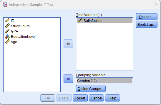
Figure 2: Independent-Samples T Test dialog with Satisfaction as the test variable and Gender as the grouping variable
Step 3: Define the Groups
Click the Define Groups button. Enter the values that represent your two groups:
- Group 1: 1 (Male)
- Group 2: 2 (Female)
These values must match the codes in your data. Check Variable View if you are unsure which numeric codes represent which categories.
Click Continue to return to the main dialog.
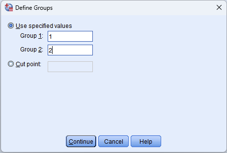
Figure 3: Define Groups dialog: Group 1 = 1 (Male), Group 2 = 2 (Female)
Step 4: Run the Test
Click OK. SPSS produces two output tables: the Group Statistics table and the Independent Samples Test table.
Interpreting the Output
Group Statistics Table
This table reports the descriptive statistics for each group separately.

Figure 4: Group Statistics table with descriptive statistics for males and females on Satisfaction
What to look at:
- N: Sample size per group (61 males, 86 females). Unequal group sizes are fine.
- Mean: The average Satisfaction score for each group. Compare these to see the direction of any difference.
- Std. Deviation: The spread of scores within each group. Similar standard deviations suggest equal variances; very different values suggest a potential Levene's test issue.
- Std. Error Mean: The standard error of each group mean. Smaller values indicate more precise estimates.
Before moving to the inferential test, note the means and standard deviations. You will need them for APA reporting and for calculating Cohen's d.
Independent Samples Test Table
This is the main results table. It contains Levene's test and the t-test results in a single table.
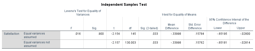
Figure 5: Independent Samples Test table with Levene's test for equality of variances and t-test results
Reading the table requires two steps:
Step A: Check Levene's test (left side of the table)
Look at the "Levene's Test for Equality of Variances" columns (F and Sig.).
- If Sig. > .05: Variances are equal. Read the top row ("Equal variances assumed").
- If Sig. < .05: Variances are unequal. Read the bottom row ("Equal variances not assumed").
Step B: Read the t-test results (right side of the table, from the correct row)
- t: The t statistic. Its absolute value tells you how many standard errors the group means are apart.
- df: Degrees of freedom. For equal variances assumed, df = N1 + N2 - 2. For Welch's t-test, df is adjusted and is often not a whole number.
- Sig. (2-tailed): The p-value. If this is below your alpha level (usually .05), the difference between groups is statistically significant.
- Mean Difference: The raw difference between the two group means (M1 - M2).
- Std. Error Difference: The standard error of that difference.
- 95% Confidence Interval: The range within which the true population mean difference likely falls. If this interval contains zero, the difference is not significant.
Putting the Output Together
In this example, Levene's test has F = 0.016, Sig. = .900 (not significant). This means variances are approximately equal, so we read the top row ("Equal variances assumed").
The t-test shows: t(145) = -2.154, p = .033, Mean Difference = -0.34.
The result is statistically significant. Females (M = 3.59, SD = 0.95) scored significantly higher than males (M = 3.25, SD = 0.94) on Satisfaction. The 95% confidence interval for the mean difference [-0.65, -0.03] does not contain zero, confirming the significant result.
Notice that the confidence interval is relatively wide compared to the mean difference itself. This tells us the estimate has some uncertainty, though we can be confident the true difference is negative (females scoring higher). The practical importance of a 0.34-point difference on a 5-point scale requires context, which is where Cohen's d comes in.
Calculating Cohen's d (Effect Size)
SPSS does not compute Cohen's d for the independent samples t-test. You need to calculate it manually. Thesis committees increasingly expect effect sizes alongside p-values, because a non-significant result with a small sample does not necessarily mean no effect exists, and a significant result with a large sample does not necessarily mean the effect is meaningful.
Formula
Where the pooled standard deviation is:
Calculation Example
Using the values from the Group Statistics table:
- (Male) = 3.2469, = 0.93843, = 61
- (Female) = 3.5869, = 0.94611, = 86
Interpretation
| Cohen's d | Effect Size | Practical Meaning |
|---|---|---|
| 0.2 | Small | Difference exists but is difficult to observe |
| 0.5 | Medium | Difference is noticeable and may be practically meaningful |
| 0.8 | Large | Difference is substantial and clearly meaningful |
Table 2: Cohen's d benchmarks for interpreting effect size (Cohen, 1988)
In this example, d = 0.36 is a small-to-medium effect. Females scored about one-third of a standard deviation higher than males on Satisfaction. Combined with the significant p-value (.033), this result provides both statistical and practical evidence of a gender difference, though the effect is modest rather than dramatic.
The sign of Cohen's d indicates direction (negative means Group 2 scored higher), but the magnitude is what matters for interpretation. Report the absolute value if the direction is clear from the means.
What to Do When Assumptions Are Violated
Normality Violation
If normality is severely violated (skewness beyond +/-2 within one or both groups), and your group sizes are below 30, the Mann-Whitney U test is the standard non-parametric alternative. It compares the ranks of scores rather than the means and does not require normality.
To run the Mann-Whitney U test in SPSS: Analyze > Nonparametric Tests > Legacy Dialogs > 2 Independent Samples. Move the test variable to the Test Variable List, the grouping variable to the Grouping Variable box, define groups, and select "Mann-Whitney U" under Test Type.
With groups of 30 or more, parametric t-tests are robust enough that moderate normality violations (skewness between -2 and +2) typically do not affect the validity of results (Glass et al., 1972). Document the violation and cite the robustness literature.
Unequal Variances (Levene's Test Significant)
This is the easiest violation to handle. Read the "Equal variances not assumed" row in the output. Welch's t-test adjusts the degrees of freedom to compensate for unequal variances. No additional test is needed.
Report it transparently: "Levene's test indicated unequal variances, F(1, 145) = 5.23, p = .024. Therefore, the Welch-adjusted t-test was used."
Both Assumptions Violated
When both normality and equal variances are violated, the Mann-Whitney U test is the safest choice. Report the violation, explain why you chose the non-parametric alternative, and present the Mann-Whitney U results using APA format.
Reporting in APA Format
Reporting the Actual Results From This Tutorial
An independent samples t-test was conducted to compare Satisfaction scores between male and female students. Levene's test for equality of variances was not significant (F = 0.02, p = .900), so equal variances were assumed. Female students (M = 3.59, SD = 0.95) reported significantly higher satisfaction than male students (M = 3.25, SD = 0.94), t(145) = -2.15, p = .033, d = 0.36, 95% CI [-0.65, -0.03]. The effect size was small to medium.
Non-Significant Result Template
If the result had been non-significant, the report would follow this structure:
An independent samples t-test was conducted to compare Satisfaction scores between male and female students. There was no significant difference between males (M = 3.25, SD = 0.94) and females (M = 3.38, SD = 0.96), t(145) = -0.84, p = .401, d = 0.14. The effect size was negligible.
With Welch's Correction (Unequal Variances)
Levene's test indicated unequal variances (F = 5.23, p = .024), so the Welch-adjusted t-test was used. There was no significant difference between males (M = 3.12, SD = 0.89) and females (M = 3.24, SD = 1.12), t(141.35) = -0.72, p = .474, d = 0.12.
APA Table Format
For thesis Results chapters that require a summary table:
| Variable | Group | N | M | SD | t | df | p | d |
|---|---|---|---|---|---|---|---|---|
| Satisfaction | Male | 61 | 3.25 | 0.94 | -2.15 | 145 | .033 | 0.36 |
| Female | 86 | 3.59 | 0.95 |
Table 3: Independent samples t-test results comparing Satisfaction by Gender
Reporting Checklist
Every independent samples t-test report should include:
- The purpose of the test (what comparison was made and why)
- Levene's test result (equal or unequal variances, and which row you read)
- Group means and standard deviations
- The t statistic, degrees of freedom, and exact p-value
- Effect size (Cohen's d) with interpretation
- The 95% confidence interval of the mean difference (optional but recommended)
Common Mistakes
1. Using the T-Test for Three or More Groups
Running multiple independent samples t-tests to compare three groups (e.g., High School vs. Bachelor's, High School vs. Master's, Bachelor's vs. Master's) inflates the Type I error rate. With three pairwise comparisons at alpha = .05, the probability of at least one false positive rises to approximately .14. Use one-way ANOVA with post-hoc tests instead.
2. Ignoring Levene's Test
Some students report only the "Equal variances assumed" row without checking whether that assumption holds. If Levene's test is significant, the degrees of freedom, p-value, and confidence interval in the top row are all incorrect. Always check and report which row you used.
3. Not Checking Normality per Group
Running a single normality test on the entire variable (both groups combined) is insufficient. The assumption requires normality within each group. Use the Factor List in the Explore procedure to test each group separately.
4. Omitting Effect Size
A p-value tells you whether the result is statistically significant, but not whether the difference is large enough to matter. A significant result with d = 0.10 and a sample of 500 is statistically significant but practically meaningless. Committees increasingly expect Cohen's d or another effect size measure.
5. Confusing Independent and Paired Designs
If the same participants are measured before and after an intervention, the observations are not independent. Using the independent samples t-test in this situation ignores the correlation between the paired measurements and produces incorrect results. Use the paired samples t-test for within-subjects comparisons.
6. Running One-Tailed Tests Without Justification
SPSS reports two-tailed p-values by default. Dividing the p-value by 2 to get a one-tailed result is only appropriate when you have a strong directional hypothesis stated before data collection. Post-hoc switching to a one-tailed test to achieve significance is a form of p-hacking that committees will question.
What Your Thesis Committee Will Ask
"Why did you use an independent samples t-test and not ANOVA?" Explain that the independent samples t-test is the appropriate test when comparing exactly two groups on a continuous outcome. ANOVA is designed for three or more groups. While one-way ANOVA with two groups produces mathematically identical results (F = t²), the t-test directly addresses the two-group comparison and is the conventional choice.
"How did you handle the assumption of equal variances?" Describe that you checked Levene's test in the SPSS output. If it was non-significant, equal variances were assumed. If significant, you used the Welch-adjusted results from the "Equal variances not assumed" row. Cite Delacre et al. (2017) if your committee questions this approach.
"The result is significant, but is the difference practically important?" This is where Cohen's d comes in. A d of 0.36 is a small-to-medium effect: females scored about one-third of a standard deviation higher than males. Whether this matters depends on the research context. In a satisfaction survey with a 1-to-5 scale, a 0.34-point difference may or may not be practically meaningful. Report the effect size, describe its magnitude using Cohen's benchmarks, and let the reader assess relevance to their specific context.
"Why should I trust the t-test if the Shapiro-Wilk test was significant?" Reference the distinction between statistical significance and practical importance in normality testing. Cite the skewness and kurtosis values (within +/-1), the Q-Q plot evidence, and the robustness literature (Schmider et al., 2010). This question is covered in depth in the normality testing guide.
Frequently Asked Questions
Next Steps
After running the independent samples t-test, the next analysis depends on your research design.
If you need to compare the same participants across two time points (pre-test vs. post-test), the paired samples t-test is the appropriate test. If your design involves three or more groups, move to one-way ANOVA, which extends the logic of the t-test to multiple comparisons with a single omnibus test.
For examining the relationship between two continuous variables rather than comparing group means, linear regression provides a framework for prediction and explanation. If your scale includes multiple items, verify its reliability with Cronbach's Alpha before using composite scores in your t-test.
Make sure your foundational analyses are documented: descriptive statistics for your sample characteristics and normality testing for assumption verification should appear in your Results chapter before the t-test results.
References
American Psychological Association. (2020). Publication manual of the American Psychological Association (7th ed.). American Psychological Association.
Cohen, J. (1988). Statistical power analysis for the behavioral sciences (2nd ed.). Lawrence Erlbaum Associates.
Delacre, M., Lakens, D., & Leys, C. (2017). Why psychologists should by default use Welch's t-test instead of Student's t-test. International Review of Social Psychology, 30(1), 92-101.
Field, A. (2018). Discovering statistics using IBM SPSS statistics (5th ed.). SAGE Publications.
Glass, G. V., Peckham, P. D., & Sanders, J. R. (1972). Consequences of failure to meet assumptions underlying the fixed effects analyses of variance and covariance. Review of Educational Research, 42(3), 237-288.
Pallant, J. (2020). SPSS survival manual (7th ed.). Open University Press.
Schmider, E., Ziegler, M., Danay, E., Beyer, L., & Bühner, M. (2010). Is it really robust? Reinvestigating the robustness of ANOVA against violations of the normal distribution assumption. Methodology, 6(4), 147-151.