Every thesis data analysis starts with descriptive statistics. Before running t-tests, ANOVA, or regression, you need to know what your data actually looks like: the means, standard deviations, distribution shapes, and whether anything unusual is going on with missing values or outliers.
SPSS gives you three separate procedures for this, and most students only know about one of them. This guide walks through all three (Descriptives, Frequencies, and Explore), shows you how to read the output, and includes APA 7th edition reporting templates for your Results chapter.
Key Takeaways:
- SPSS offers three procedures for descriptive statistics: Descriptives (quick numeric summaries), Frequencies (categorical data and frequency counts), and Explore (in-depth analysis with normality tests and plots)
- Skewness values between -1 and +1 suggest approximate normality; values beyond -2 or +2 indicate substantial deviation
- Report mean and SD for normally distributed continuous variables; report median and IQR for skewed data or ordinal variables
- The Explore procedure is the most thorough option, producing confidence intervals, Shapiro-Wilk tests, boxplots, and Q-Q plots in a single run
- Always report descriptive statistics before inferential analyses in your thesis Results chapter
Before you begin: This guide assumes you have SPSS installed and your data entered in the Data View with variables properly defined in Variable View. If you need to check the reliability of a multi-item scale before summarizing it, see our guide on Cronbach's Alpha in SPSS.
Example Dataset
This tutorial uses a sample thesis dataset with 150 respondents that you can download from the sidebar and follow along. The dataset includes six variables commonly found in social science thesis research:
- Satisfaction (Scale, 1.00 to 5.00) and GPA (Scale, 1.80 to 4.00): continuous variables with approximately normal distributions, used for the Descriptives and Explore procedures
- StudyHours (Scale, 3.40 to 35.00): a continuous variable with a right-skewed distribution and two mild outliers, useful for demonstrating how skewness appears in SPSS output and how outliers show up in Explore boxplots
- Gender (Nominal, 1 = Male, 2 = Female) and EducationLevel (Ordinal, 1 = High School, 2 = Bachelor's, 3 = Master's): categorical variables used for the Frequencies procedure
- Age (Scale, 18 to 40): an additional continuous variable for variety in the Descriptives output
The dataset intentionally includes 2 to 3 missing values per variable so you can see how SPSS handles missing data in the output (the Valid N column).
If you open the .sav file, the variables are already configured in Variable View with the correct measurement levels and value labels. If you imported the .xlsx version instead, you will need to set these manually. Switch to Variable View (tab at the bottom of the SPSS window) and verify the following:
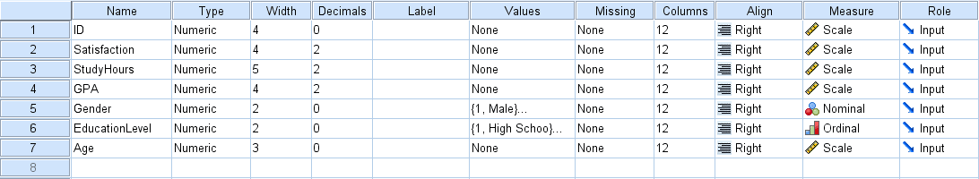
Figure 1: Variable View configuration: Satisfaction, StudyHours, GPA, and Age set to Scale; Gender set to Nominal with value labels (1 = Male, 2 = Female); EducationLevel set to Ordinal with value labels (1 = High School, 2 = Bachelor's, 3 = Master's)
Getting the measurement level right matters. If a continuous variable is incorrectly set to Nominal, some SPSS procedures will exclude it or produce meaningless results. If a categorical variable is left as Scale, SPSS will compute a mean for it without warning (see Common Mistake #1 below).
What Are Descriptive Statistics?
Descriptive statistics summarize your dataset without making inferences about a larger population. They answer the most basic questions about your variables: what is the average? How spread out are the values? Is the distribution symmetric or lopsided?
These measures fall into four categories:
Central tendency tells you where the middle of your data is. The mean (arithmetic average) is the most common, followed by the median (the middle value when sorted) and mode (the most frequent value). Which one you report depends on your distribution shape.
Dispersion (variability) captures how spread out the values are. Standard deviation is the workhorse here, but you will also encounter the range, variance, and interquartile range (IQR) in SPSS output.
Distribution shape describes whether your data is symmetric or skewed. Skewness quantifies asymmetry, while kurtosis measures how heavy or light the tails are compared to a normal distribution. Both matter for deciding which inferential tests are appropriate.
Position locates specific values relative to the rest of the data: percentiles, quartiles, and z-scores.
Why Descriptive Statistics Matter for Your Thesis
For thesis work specifically, descriptive statistics do three things that your committee will expect to see:
First, they characterize your sample. Your readers need to know who participated, what the score distributions look like, and whether anything stands out. This section typically opens your Results chapter or closes your Methods chapter.
Second, they screen your assumptions. T-tests, ANOVA, and regression all assume approximate normality. Skewness, kurtosis, and the visual plots from SPSS help you evaluate whether those assumptions hold before you run the actual tests.
Third, they reveal data quality issues. Missing values, outliers, impossible scores (a 6 on a 1-5 Likert scale), and unexpected patterns all show up in descriptive output. Catching these problems early saves you from running analyses on flawed data.
Which SPSS Procedure Should You Use?
SPSS has three procedures under Analyze > Descriptive Statistics, and they are not interchangeable. Most thesis analyses require at least two of them.
| Procedure | Best For | Output Includes | Use When |
|---|---|---|---|
| Descriptives | Quick numeric summaries of continuous variables | Mean, SD, min, max, variance, skewness, kurtosis | You need a compact summary table for several numeric variables at once |
| Frequencies | Categorical data and frequency distributions | Frequency tables, percentages, cumulative percentages, mean, median, mode | You have nominal/ordinal variables, or you need the median and mode for continuous variables |
| Explore | In-depth variable investigation | Confidence intervals, normality tests (Shapiro-Wilk, K-S), boxplots, stem-and-leaf, Q-Q plots, outlier identification | You need to check normality assumptions, identify outliers, or produce publication-quality plots |
Table 1: Comparison of the three SPSS descriptive statistics procedures
For a typical thesis, run Descriptives first to get a quick overview of your continuous variables. Then run Frequencies for any categorical or ordinal variables. Finally, use Explore on your key continuous variables to check normality and identify outliers before moving to inferential tests.
Procedure 1: Descriptives (Quick Numeric Summary)
Descriptives is the simplest of the three. It computes basic summary statistics for continuous (scale) variables and displays them all in one output table. If you need a compact overview of several variables side by side, start here.
Step 1: Open the Descriptives Dialog
Navigate to Analyze > Descriptive Statistics > Descriptives from the top menu.
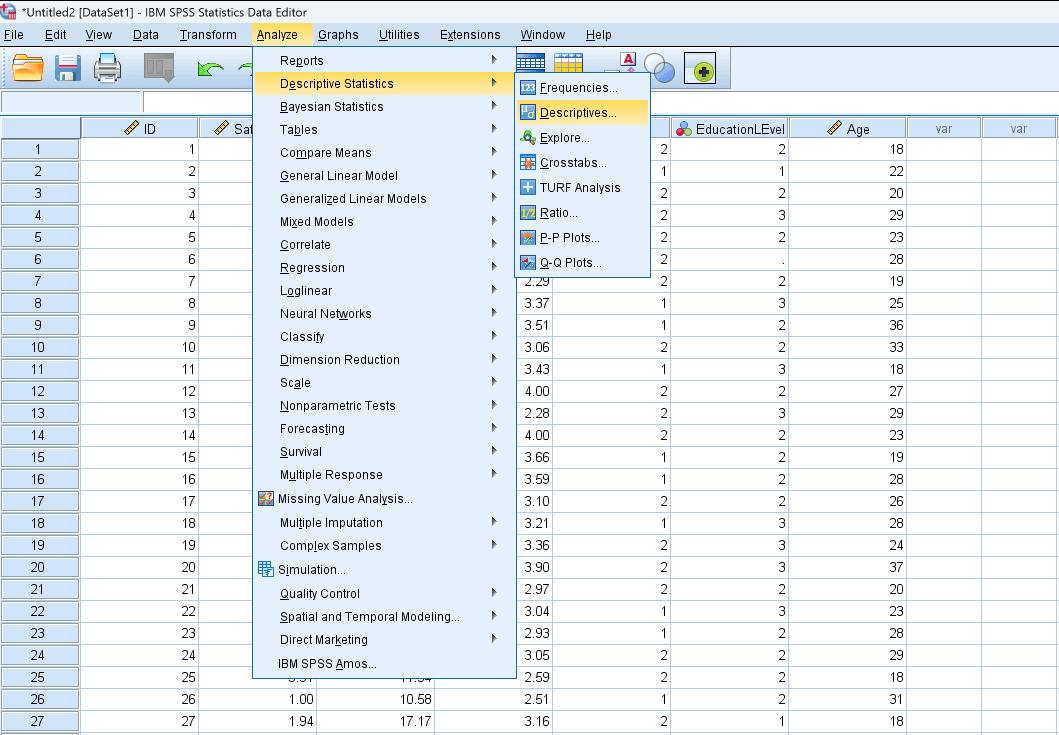
Figure 2: Navigating to the Descriptives procedure in SPSS
Step 2: Select Your Variables
In the Descriptives dialog box, move the continuous variables you want to summarize from the left panel to the Variable(s) list on the right. You can select multiple variables at once by holding Ctrl (Cmd on Mac) and clicking each variable, then clicking the arrow button.
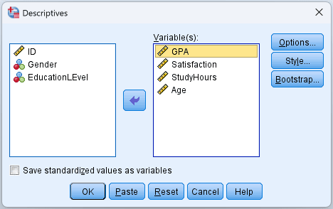
Figure 3: The Descriptives dialog box with variables moved to the Variable(s) list
Step 3: Configure Options
Click the Options button to customize which statistics SPSS calculates. By default, SPSS computes the mean, standard deviation, minimum, and maximum. In the Options dialog, you can additionally enable:
- Variance (the square of the standard deviation)
- Range (maximum minus minimum)
- S.E. mean (standard error of the mean)
- Skewness (distribution symmetry)
- Kurtosis (tail weight relative to normal)
For thesis work, enable Skewness and Kurtosis at minimum. These values are essential for assessing whether your data approximates a normal distribution, which most parametric tests require.
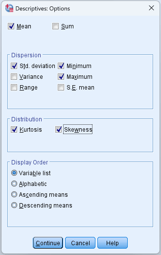
Figure 4: Descriptives Options dialog with skewness and kurtosis enabled
Click Continue to return to the main dialog, then click OK to run the analysis.
Step 4: Interpret the Output
SPSS produces a single Descriptive Statistics table with one row per variable.
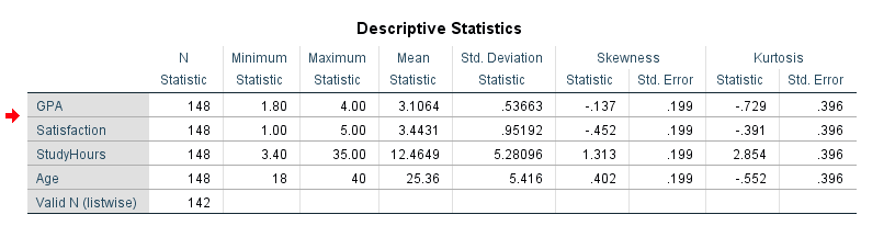
Figure 5: Descriptive Statistics output table in SPSS
How to read each column:
- N is the number of valid (non-missing) cases. Compare this to your expected sample size. If the numbers differ, you have missing data that needs to be addressed.
- Minimum / Maximum show the smallest and largest observed values. Check these against your expected data range. A score of 6 on a 1-5 Likert scale, for example, signals a data entry error.
- Mean is the arithmetic average. For normally distributed data, this is the best measure of central tendency.
- Std. Deviation quantifies how far observations typically fall from the mean. A very large SD relative to the mean often points to high variability or outliers pulling the distribution.
- Skewness measures distribution asymmetry. See the interpretation guide below.
- Kurtosis measures tail heaviness. See the interpretation guide below.
Procedure 2: Frequencies (Categorical Data and Counts)
Frequencies is what you need for categorical variables (gender, education level, treatment group) and for any situation where you want counts and percentages. It also computes the median and mode for continuous variables, which Descriptives does not provide. If you have Likert scale items and want to see how responses distribute across the scale, this is the procedure to use.
Step 1: Open the Frequencies Dialog
Navigate to Analyze > Descriptive Statistics > Frequencies.
Step 2: Select Variables and Configure Statistics
Move your variables to the Variable(s) list. Click the Statistics button to choose which summary measures to compute.
For categorical variables (nominal/ordinal), the default frequency table is typically sufficient. You may also enable the Mode to identify the most common category.
For continuous variables where you need the median, check the following under Statistics:
- Mean, Median, Mode (under Central Tendency)
- Std. Deviation, Variance, Range (under Dispersion)
- Skewness, Kurtosis (under Distribution)
- Quartiles or specific Percentile(s) if needed
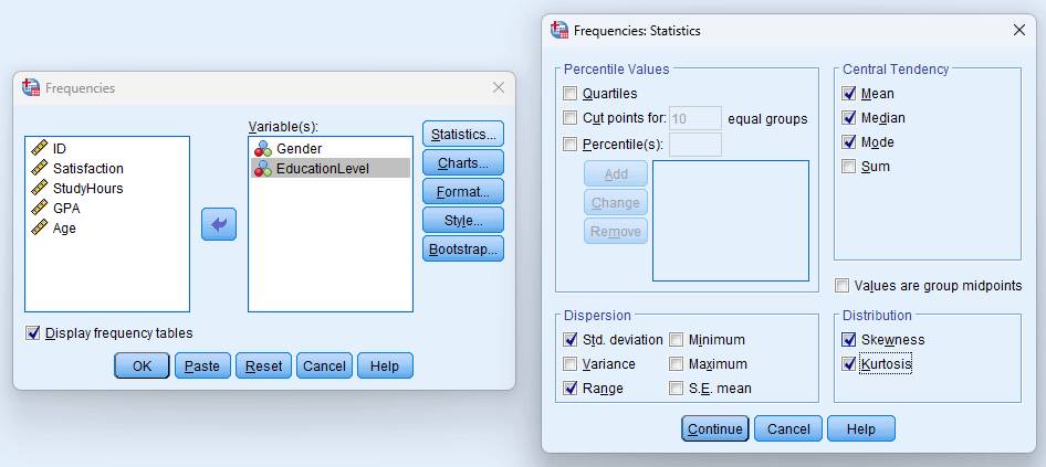
Figure 6: Frequencies Statistics dialog with recommended options for thesis analysis
Step 3: Interpret the Output
Frequencies produces two types of output:
Statistics table: A summary table showing the measures you selected (mean, median, mode, SD, skewness, kurtosis, valid N, missing N).
Frequency table(s): One table per variable showing each unique value, its frequency (count), percent, valid percent (excluding missing), and cumulative percent.
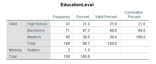
Figure 7: Frequency table output for a categorical variable
Key points for interpretation:
- Percent includes missing values in the denominator; Valid Percent excludes them. Report Valid Percent in your thesis because it reflects the actual distribution among respondents who answered.
- Cumulative Percent shows the running total. This is useful for ordinal data: "73% of respondents rated satisfaction 4 or below on a 5-point scale."
- For Likert scale items, the frequency table is often more informative than the mean alone. A mean of 3.5 looks different when 80% of respondents chose 3 or 4 versus when responses split between 1 and 5.
Procedure 3: Explore (In-Depth Analysis)
Explore is the most powerful of the three and the one your committee is most likely to ask about. It produces normality tests (Shapiro-Wilk and Kolmogorov-Smirnov), confidence intervals, outlier tables, and publication-quality plots (histograms, boxplots, Q-Q plots) in a single run.
Step 1: Open the Explore Dialog
Navigate to Analyze > Descriptive Statistics > Explore.
Step 2: Configure the Analysis
- Move your continuous variables to the Dependent List.
- Optionally, move a categorical grouping variable to the Factor List if you want descriptive statistics broken down by group (e.g., descriptive statistics for males vs. females).
- In the Display section at the bottom, select Both to generate both statistics and plots.
Step 3: Configure Plots and Statistics
Click Plots to configure visual output. For thesis work, enable:
- Histogram (with normal curve overlay)
- Normality plots with tests (produces Shapiro-Wilk and Kolmogorov-Smirnov tests, plus Q-Q plots)
Click Statistics to confirm that:
- Descriptives is checked (provides mean, median, variance, SD, min, max, range, IQR, skewness, kurtosis, and 95% confidence interval for the mean)
- Outliers is checked (identifies the five largest and five smallest values)
- Percentiles is checked if you need quartile or percentile values
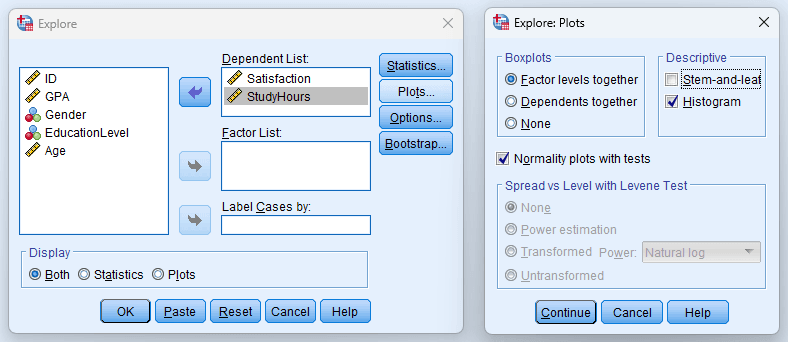
Figure 8: Explore Plots dialog with recommended settings for thesis analysis
Step 4: Interpret the Output
The Explore procedure produces several output sections:
Descriptives table: Includes the mean (with 95% confidence interval), 5% trimmed mean, median, variance, standard deviation, minimum, maximum, range, interquartile range, skewness, and kurtosis.
Pay attention to the 5% trimmed mean. SPSS removes the top and bottom 5% of cases and recalculates the mean. If the trimmed mean differs noticeably from the regular mean, outliers are pulling your average in one direction.
Tests of Normality table: Contains the Kolmogorov-Smirnov (K-S) and Shapiro-Wilk test results. The Shapiro-Wilk test is preferred for samples under 50. A significant result (p < .05) indicates the distribution significantly deviates from normality.
Boxplots: Identify outliers (circles) and extreme values (asterisks). Cases that appear as outliers in the boxplot warrant investigation.
Q-Q Plot: Points falling along the diagonal line suggest normality. Systematic deviations from the line indicate non-normality.
How to Interpret Skewness and Kurtosis
These two values show up in both the Descriptives and Explore output, and they determine whether you can proceed with parametric tests or need to consider alternatives.
Skewness Interpretation
| Skewness Value | Interpretation | Implication |
|---|---|---|
| Approximately 0 | Symmetric distribution | Data is approximately normally distributed (good) |
| Positive (> 0) | Right-skewed (positive skew) | Tail extends to the right; most values cluster on the left |
| Negative (< 0) | Left-skewed (negative skew) | Tail extends to the left; most values cluster on the right |
| Between -1 and +1 | Approximately normal | Acceptable for most parametric tests |
| Between -2 and +2 | Moderately skewed | Acceptable with caution; some tests are robust to this level |
| Beyond -2 or +2 | Substantially skewed | Consider data transformation or non-parametric alternatives |
Table 2: Skewness value interpretation guide
Kurtosis Interpretation
SPSS reports excess kurtosis, which means the normal distribution has a kurtosis value of 0 (not 3, which is the mathematical kurtosis of a normal distribution).
| Kurtosis Value | Interpretation | Implication |
|---|---|---|
| Approximately 0 | Mesokurtic (normal peakedness) | Tails are similar to a normal distribution |
| Positive (> 0) | Leptokurtic (heavy tails) | More extreme values than a normal distribution; potential outliers |
| Negative (< 0) | Platykurtic (light tails) | Fewer extreme values than a normal distribution |
| Between -1 and +1 | Approximately normal | Acceptable for parametric tests |
| Beyond -2 or +2 | Substantially non-normal | Investigate outliers; consider transformation |
Table 3: Kurtosis value interpretation guide
As a practical rule: if both skewness and kurtosis fall within -1 to +1, proceed with parametric tests. If either value exceeds -2 or +2, consider data transformation (log, square root) or switch to non-parametric alternatives. Values between -1 and -2 (or +1 and +2) are a judgment call that depends on your sample size and the robustness of your chosen test.
Reporting Descriptive Statistics in APA Format
APA 7th edition has specific conventions for reporting descriptive statistics. The templates below are designed to be adapted directly for your thesis Results chapter.
APA Template for Continuous Variables
At minimum, report the sample size, mean, and standard deviation for each continuous variable. If your committee expects normality documentation (most do), include skewness and kurtosis as well.
In-text reporting:
Participants' satisfaction scores ranged from 1.00 to 5.00 (M = 3.44, SD = 0.95, N = 148). The distribution was approximately normal (skewness = -0.45, kurtosis = -0.39).
Table format (recommended for multiple variables):
| Variable | N | M | SD | Min | Max | Skewness | Kurtosis |
|---|---|---|---|---|---|---|---|
| Satisfaction | 148 | 3.44 | 0.95 | 1.00 | 5.00 | -0.45 | -0.39 |
| Study Hours | 148 | 12.46 | 5.28 | 3.40 | 35.00 | 1.31 | 2.85 |
| GPA | 148 | 3.11 | 0.54 | 1.80 | 4.00 | -0.14 | -0.73 |
Table 4: Example APA-formatted descriptive statistics table
APA formatting reminders:
- Italicize statistical symbols: M, SD, N, n
- Two decimal places for most statistics
- Table values are not bolded; only the header row is
- Number your tables sequentially ("Table 1", "Table 2") with a descriptive title above each
- Descriptive statistics tables go early in your Results section, before inferential analyses
APA Template for Categorical Variables
For categorical variables, report frequencies and percentages.
In-text reporting:
The sample consisted of 87 females (58.4%) and 62 males (41.6%). The majority of participants held a bachelor's degree (n = 71, 48.0%), followed by master's degree (n = 45, 30.4%) and high school diploma (n = 32, 21.6%).
Table format:
| Variable | Category | n | % |
|---|---|---|---|
| Gender | Female | 87 | 58.4 |
| Male | 62 | 41.6 | |
| Education | High School | 32 | 21.6 |
| Bachelor's | 71 | 48.0 | |
| Master's | 45 | 30.4 |
Table 5: Example APA-formatted frequency table for categorical variables
Where Descriptive Statistics Appear in a Thesis
Descriptive statistics typically appear in one of two locations:
-
End of the Methods chapter (sample demographics). Report the characteristics of your sample: gender breakdown, age range, education level, and other relevant demographic variables.
-
Beginning of the Results chapter (variable summaries). Report the descriptive statistics for your research variables (means, standard deviations, distribution properties) before presenting inferential test results.
Some thesis committees prefer all descriptive statistics in the Results chapter. Confirm the expected placement with your supervisor.
Common Mistakes When Running Descriptive Statistics in SPSS
1. Using Descriptives for Categorical Variables
If gender is coded as 1 = Male and 2 = Female, SPSS will compute a mean of 1.58 without any complaint. That number is meaningless. Descriptives computes means and standard deviations, which only make sense for continuous variables. Use Frequencies for categorical data.
2. Ignoring the Valid N
SPSS reports the number of valid (non-missing) cases as N in the output. If your dataset has 200 cases but a variable shows N = 185, 15 values are missing. Always check valid N and report missing data in your thesis.
3. Reporting Only the Mean Without Variability
A mean satisfaction score of 3.5 could come from a sample where everyone scored between 3 and 4, or from one where half the respondents scored 1 and half scored 5. The mean alone does not tell you which. Always pair it with the standard deviation.
4. Not Checking Skewness Before Parametric Tests
Many students proceed directly from descriptive statistics to t-tests or ANOVA without verifying normality. If your data is substantially skewed (beyond +/-2), parametric test results may be unreliable. The Explore procedure makes this check straightforward by producing both numeric tests and visual plots.
5. Confusing Percent and Valid Percent in Frequency Tables
SPSS reports both Percent (includes missing values in the denominator) and Valid Percent (excludes missing values). In your thesis, report Valid Percent because it represents the distribution among respondents who actually answered the question.
6. Reporting Too Many Decimal Places
SPSS output often displays eight or more decimal places. Copying M = 3.4527189 directly into your thesis looks unprofessional and implies a level of precision your measurement instrument almost certainly does not have. APA recommends two decimal places: M = 3.45.
7. Running Descriptives Without Checking Variable Measurement Level
SPSS uses the measurement level defined in Variable View (Nominal, Ordinal, Scale) to determine which statistics are appropriate. If your continuous variable is incorrectly set to Nominal, some procedures may exclude it. Verify measurement levels in Variable View before running any analysis.
What Your Thesis Committee Will Ask
These questions come up in nearly every thesis defense that involves quantitative data:
"How do you know your data is normally distributed?" This is where your Explore output earns its value. Point to the skewness and kurtosis values, the Shapiro-Wilk test results, and the Q-Q plot. State the threshold you applied: "Skewness and kurtosis values fell within the acceptable range of -1 to +1 for all study variables, and the Q-Q plots showed no systematic deviation from normality."
"Why did you choose mean and SD rather than median and IQR?" The answer should demonstrate that you made a deliberate choice, not a default one. Explain that you assessed distribution shape first and that the data was approximately normal, which justified the use of parametric summary measures.
"How much missing data do you have, and how did you handle it?" Your descriptive output already contains this information in the valid N column. State the percentage of missing data per variable and explain your handling strategy (listwise deletion, pairwise deletion, or imputation) with justification.
"Are there any outliers in your data?" Reference the boxplots and Extreme Values table from Explore. If you identified outliers, explain whether you retained or excluded them, and why. Committees want to see that you investigated rather than ignored potential problems.
Frequently Asked Questions
Next Steps After Descriptive Statistics
With your descriptive output reviewed, the next steps depend on what you found:
If skewness or kurtosis flagged potential non-normality, run formal normality tests. Our guide on how to check normality in SPSS walks through Shapiro-Wilk, Q-Q plots, and what to do when normality fails. The Explore procedure already produces these tests, but if you skipped Explore, you will need to do this before any parametric test.
If your variables are multi-item scales (e.g., a satisfaction scale composed of 5 Likert items), check their reliability using Cronbach's Alpha in SPSS before computing composite scores.
Once your data is clean and assumptions are verified, move to hypothesis testing. The specific test depends on your research design:
- Comparing two group means: Independent samples t-test or paired samples t-test
- Comparing three or more groups: One-way ANOVA or repeated measures ANOVA
- Examining relationships between continuous variables: Correlation or linear regression in SPSS
- Testing mediation hypotheses: Mediation analysis in SPSS
- Testing moderation hypotheses: Moderation analysis in SPSS
References
American Psychological Association. (2020). Publication manual of the American Psychological Association (7th ed.). American Psychological Association.
Field, A. (2018). Discovering statistics using IBM SPSS statistics (5th ed.). SAGE Publications.
George, D., & Mallery, P. (2019). IBM SPSS statistics 26 step by step: A simple guide and reference (16th ed.). Routledge.
Hair, J. F., Babin, B. J., Anderson, R. E., & Black, W. C. (2019). Multivariate data analysis (8th ed.). Cengage Learning.
Pallant, J. (2020). SPSS survival manual (7th ed.). Open University Press.
Tabachnick, B. G., & Fidell, L. S. (2019). Using multivariate statistics (7th ed.). Pearson.