Normality testing is one of the most common steps thesis committees expect to see before any parametric analysis. T-tests, ANOVA, Pearson correlation, and linear regression all assume that the data (or the residuals) are approximately normally distributed. Skipping this step is one of the most frequent criticisms in thesis defenses.
SPSS provides four methods for checking normality: the Shapiro-Wilk test, the Kolmogorov-Smirnov test, Q-Q plots, and histograms with normal curves. This guide covers all four, explains how to interpret the output, and shows what to do when your data fails the normality assumption.
Key Takeaways:
- Use the Explore procedure (Analyze > Descriptive Statistics > Explore) to run all normality checks in one step: Shapiro-Wilk, K-S, histograms, and Q-Q plots
- The Shapiro-Wilk test is more powerful than Kolmogorov-Smirnov and is preferred for most thesis work (samples up to 2,000)
- A significant test (p < .05) means the data deviates from normality, but practical severity matters more than the p-value, especially in large samples
- Skewness between -1 and +1 generally indicates acceptable normality for parametric tests; values beyond +/-2 indicate a serious problem
- When normality fails, you have three options: non-parametric alternatives, data transformations, or proceeding with justification (robust parametric tests)
Before you begin: This guide assumes you have your data loaded in SPSS with variables properly defined in Variable View. If you have not run descriptive statistics yet, start with our guide on descriptive statistics in SPSS. You should also verify that your continuous variables have the measurement level set to Scale in Variable View.
Why Normality Matters for Your Thesis
Parametric statistical tests (t-tests, ANOVA, Pearson correlation, linear regression) rely on the assumption that the data follows a roughly bell-shaped, symmetric distribution. When this assumption is severely violated, the p-values produced by these tests can be inaccurate, leading to incorrect conclusions about your hypotheses.
The practical question for thesis work is not whether your data is perfectly normal. No real-world dataset is. The question is whether the deviation from normality is severe enough to compromise your analysis. This distinction matters because:
Parametric tests are robust to moderate violations. Research consistently shows that t-tests and ANOVA perform well even when the normality assumption is modestly violated, particularly with sample sizes above 30 (Glass, Peckham, & Sanders, 1972; Schmider et al., 2010). A slightly skewed distribution will not invalidate your results.
With large samples, formal tests become overly sensitive. The Shapiro-Wilk test will flag a trivial deviation from normality as "significant" when you have 300 or more cases, even though the deviation has zero practical impact on your parametric test results.
With small samples, formal tests lack power. When you have fewer than 20 cases, both the Shapiro-Wilk and K-S tests may fail to detect genuinely non-normal distributions. Visual methods become essential.
This is why experienced researchers use multiple methods together rather than relying on a single test or a single threshold.
Which Normality Method to Use
SPSS offers several approaches to assessing normality. Each has strengths and limitations, and your thesis is strongest when you combine at least two.
| Method | Type | Strengths | Limitations | Best For |
|---|---|---|---|---|
| Shapiro-Wilk | Statistical test | Most powerful formal test; widely recommended | Overly sensitive in large samples (n > 300); limited to n < 2,000 | Primary formal test for most thesis work |
| Kolmogorov-Smirnov (Lilliefors) | Statistical test | No upper sample size limit | Low power in small samples; less sensitive than Shapiro-Wilk | Secondary test; required by some committees |
| Q-Q Plot | Visual | Shows exactly where and how the distribution deviates; unaffected by sample size | Requires subjective interpretation | Essential complement to formal tests |
| Histogram | Visual | Intuitive; reveals distribution shape, gaps, and clusters | Hard to judge with small samples; bin width affects appearance | Quick initial screening |
| Skewness/Kurtosis | Numeric | Simple thresholds; easy to report | No formal hypothesis test; thresholds are conventions, not rules | Supplementary evidence for APA reporting |
Table 1: Comparison of normality assessment methods in SPSS
Recommended approach for thesis work: Run the Shapiro-Wilk test as your primary formal test, inspect the Q-Q plot for visual confirmation, and report skewness/kurtosis values as supplementary evidence. Include histograms in your appendix if your committee wants to see the distribution shapes.
Example Dataset
This tutorial uses the same thesis dataset from our descriptive statistics guide. You can download it from the sidebar. The dataset includes 150 respondents with variables specifically designed to demonstrate both normal and non-normal distributions:
- Satisfaction (Scale, 1.00 to 5.00): approximately normally distributed based on skewness and kurtosis, though the Shapiro-Wilk test flags it as significant due to sample size sensitivity.
- StudyHours (Scale, 3.40 to 35.00): right-skewed with two mild outliers. This variable has genuine normality violations visible in both the test statistics and the visual output.
- GPA (Scale, 1.80 to 4.00): approximately normally distributed.
- Age (Scale, 18 to 40): approximately normally distributed.
Working with both normal and non-normal variables in the same analysis is intentional. It also creates the exact scenario most thesis students encounter: a significant Shapiro-Wilk result that does not necessarily mean the data is unusable for parametric tests.
Step-by-Step: Running Normality Tests in SPSS
The Explore procedure is the most efficient way to check normality because it produces all four methods (Shapiro-Wilk, K-S, Q-Q plots, and histograms) in a single run.
Step 1: Open the Explore Dialog
Go to Analyze > Descriptive Statistics > Explore.

Figure 1: Navigate to Analyze > Descriptive Statistics > Explore in the SPSS menu
Step 2: Select Your Variables
Move the continuous variables you want to test into the Dependent List box. For this tutorial, move Satisfaction, StudyHours, GPA, and Age into the Dependent List.
Do not include categorical variables (Gender, EducationLevel) in the Dependent List. Normality testing applies to continuous variables only.
If you need to test normality within groups (for example, Satisfaction scores for males and females separately), add the grouping variable to the Factor List box. This is important when your subsequent analysis compares groups, because the normality assumption applies within each group.

Figure 2: Explore dialog with Satisfaction, StudyHours, GPA, and Age in the Dependent List
Step 3: Enable Normality Plots
Click the Plots button in the Explore dialog. In the Plots sub-dialog:
- Check Normality plots with tests. This enables the Shapiro-Wilk and Kolmogorov-Smirnov tests along with Q-Q plots.
- Under Boxplots, keep Factor levels together selected (the default).
- Optionally check Histogram if you want histograms included in the output.
Click Continue to return to the main dialog.
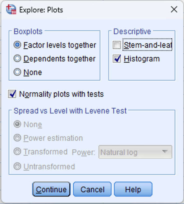
Figure 3: Explore Plots dialog: check "Normality plots with tests" and optionally "Histogram"
Step 4: Run the Analysis
Click OK in the main Explore dialog. SPSS will produce the output in the Output Viewer, including:
- A Descriptives table (with skewness and kurtosis values)
- The Tests of Normality table (Shapiro-Wilk and Kolmogorov-Smirnov)
- Normal Q-Q plots for each variable
- Detrended Normal Q-Q plots
- Histograms (if selected)
- Boxplots
Interpreting the Output
The Tests of Normality Table
This is typically the first table your committee will look at. SPSS produces both the Kolmogorov-Smirnov (with Lilliefors correction) and Shapiro-Wilk test results side by side.
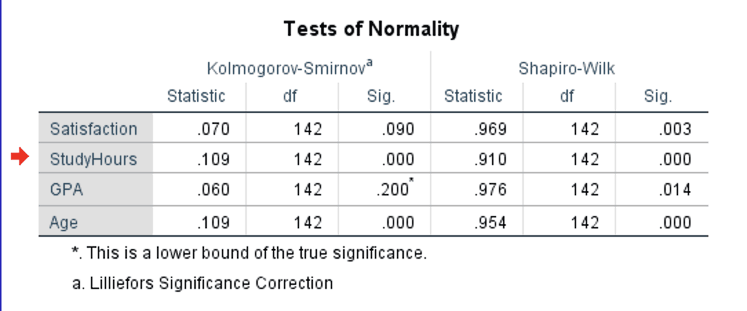
Figure 4: Tests of Normality table with Kolmogorov-Smirnov and Shapiro-Wilk results for all four variables
How to read this table:
- Statistic: The test statistic value. For Shapiro-Wilk, values closer to 1.000 indicate stronger normality. For K-S, smaller values indicate better fit to a normal distribution.
- df: Degrees of freedom (equals your sample size for each variable, minus any missing cases).
- Sig.: The p-value. This is the number that determines your conclusion.
Decision rule:
- If Sig. > .05: The data does not significantly deviate from normality. You can proceed with parametric tests.
- If Sig. < .05: The data significantly deviates from normality. Further investigation is needed (check the severity using skewness/kurtosis and Q-Q plots).
In the example output, notice that all four variables have significant Shapiro-Wilk results (p < .05). This is a common scenario with samples of 100 or more cases, and it illustrates why you should never rely on the p-value alone.
The critical distinction is between statistically significant and practically important deviations. StudyHours (W = .910, p < .001) is genuinely non-normal with a skewness of 1.39 and kurtosis of 3.05. But Satisfaction (W = .969, p = .003), GPA (W = .976, p = .014), and Age (W = .954, p < .001) all have skewness and kurtosis values well within the -1 to +1 range. The Shapiro-Wilk test detected trivial deviations in these three variables that have no practical impact on parametric test results. The Q-Q plots and skewness/kurtosis values (covered below) confirm this.
Also notice that the K-S test tells a different story: Satisfaction (p = .090) and GPA (p = .200) are non-significant, while StudyHours (p < .001) and Age (p < .001) are significant. This demonstrates the power difference between the two tests. K-S missed the minor deviations that Shapiro-Wilk detected.
Which test to report? Use the Shapiro-Wilk result as your primary test. It is more powerful (better at detecting non-normality) and is recommended by most statistics textbooks (Field, 2018; Pallant, 2020). Report the K-S result alongside it if your committee or journal requires both. But always supplement the formal test with skewness/kurtosis values and Q-Q plots, as this example demonstrates.
The Q-Q Plot
The Normal Q-Q plot (quantile-quantile plot) graphs the expected values from a normal distribution on the X-axis against the observed values from your data on the Y-axis. If the data is perfectly normal, all points fall on the diagonal line.
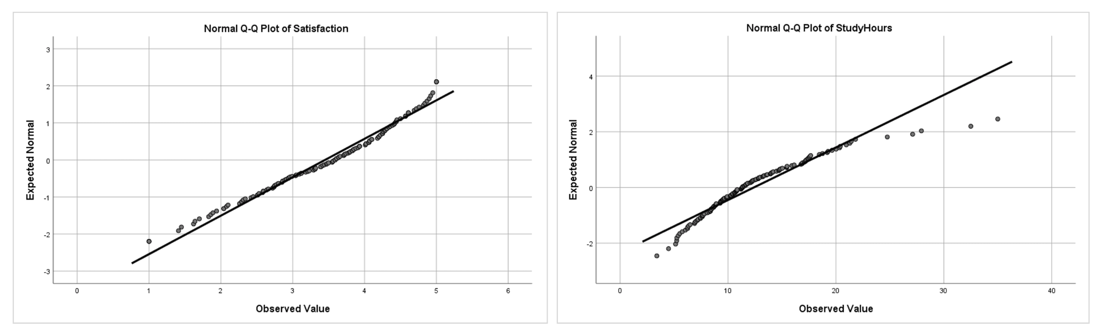
Figure 5: Q-Q plots side by side: Satisfaction (left) follows the diagonal closely, indicating approximate normality; StudyHours (right) curves away at the upper end, indicating right skew
How to interpret Q-Q plots:
- Points on or near the line: Data is approximately normal. Minor scatter around the line is expected and acceptable.
- Systematic curve (S-shape or banana shape): Data is skewed. An upward curve at the right end indicates right skew (as with StudyHours). A downward curve at the left end indicates left skew.
- Points departing at both ends: Heavy tails (leptokurtic distribution). Points fall below the line at the left and above it at the right.
- Individual points far from the line: Potential outliers. If only one or two points at the extremes deviate substantially, these are likely outliers rather than evidence of non-normality in the overall distribution.
Q-Q plots are particularly valuable for large samples where the Shapiro-Wilk test may be overly sensitive. A Q-Q plot that looks reasonably straight is strong evidence that your data is acceptable for parametric tests, even if the formal test produces a significant p-value.
Histograms with Normal Curve
Histograms provide an intuitive view of your distribution's shape. SPSS overlays a normal curve on the histogram when you request it through the Explore procedure.
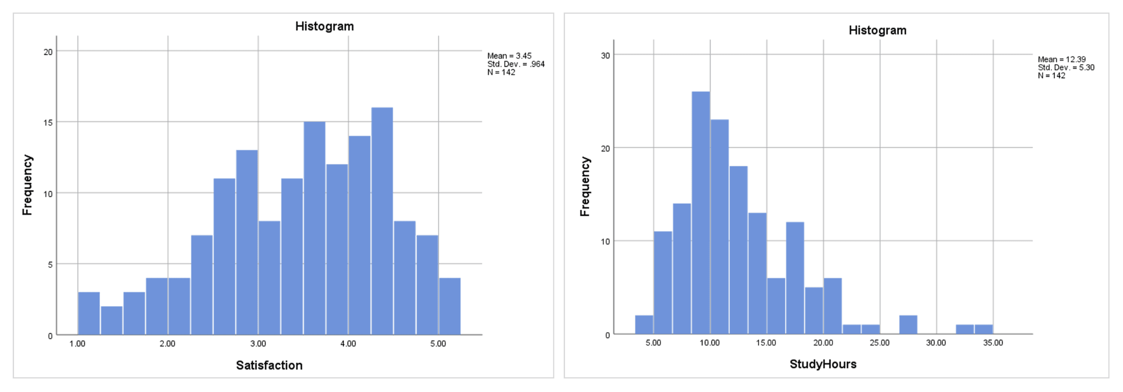
Figure 6: Histograms side by side: Satisfaction (left) shows a roughly symmetric distribution; StudyHours (right) is visibly right-skewed with a long tail
Histograms are best used for initial screening rather than formal assessment. They are affected by bin width (the number of bars), and with small samples the shape can look irregular even when the underlying distribution is normal. Use them alongside Q-Q plots and formal tests, not as your sole method.
Skewness and Kurtosis Values
The Explore procedure includes skewness and kurtosis in the Descriptives table (the same table that contains means and standard deviations). If you already ran descriptive statistics on these variables, you have these values from the earlier output.
| Variable | Skewness (SE) | Kurtosis (SE) | Interpretation |
|---|---|---|---|
| Satisfaction | -0.477 (0.203) | -0.409 (0.404) | Within +/-1: approximately normal |
| StudyHours | 1.392 (0.203) | 3.053 (0.404) | Skewness > 1: right-skewed; kurtosis > 2: heavy tails |
| GPA | -0.161 (0.203) | -0.718 (0.404) | Within +/-1: approximately normal |
| Age | 0.415 (0.203) | -0.500 (0.404) | Within +/-1: approximately normal |
Table 2: Skewness and kurtosis values from the Explore descriptive output
Interpretation thresholds:
| Range | Skewness Interpretation | Kurtosis Interpretation | Action |
|---|---|---|---|
| -1 to +1 | Approximately symmetric | Approximately normal tails | Safe for parametric tests |
| -2 to -1 or +1 to +2 | Moderately skewed | Moderately non-normal tails | Usually acceptable, especially with n > 30 |
| Beyond +/-2 | Substantially skewed | Substantially non-normal tails | Consider non-parametric tests or transformations |
Table 3: Skewness and kurtosis interpretation thresholds for normality assessment
Note that these thresholds are conventions, not absolute rules. Different sources recommend different cutoffs. George and Mallery (2019) use +/-1 for "excellent" and +/-2 for "acceptable." Hair et al. (2019) consider values beyond +/-1.96 as significant at the .05 level for samples over 50. The key point is to state which threshold you applied in your thesis and apply it consistently across all variables.
What to Do When Normality Fails
When one or more variables fail normality testing, you have three options. The best choice depends on how severely the distribution deviates and which analysis you plan to run.
Option 1: Use Non-Parametric Alternatives
Non-parametric tests do not assume normality and are the most straightforward solution when the violation is severe.
| Parametric Test | Non-Parametric Alternative | When to Switch |
|---|---|---|
| Independent samples t-test | Mann-Whitney U test | Severe skewness or small sample with non-normal data |
| Paired samples t-test | Wilcoxon signed-rank test | Severe skewness in the difference scores |
| One-way ANOVA | Kruskal-Wallis H test | Severe skewness in one or more groups |
| Pearson correlation | Spearman rank correlation | Non-linear relationship or ordinal data |
Table 4: Parametric tests and their non-parametric alternatives
Option 2: Transform the Data
Data transformations can reduce skewness and bring a variable closer to a normal distribution. Common transformations in SPSS:
For right-skewed data (positive skewness):
- Log transformation: Transform > Compute Variable >
LN(variable). Best for moderate right skew. - Square root transformation: Transform > Compute Variable >
SQRT(variable). Milder correction than log.
For left-skewed data (negative skewness):
- Reflect and log: Transform > Compute Variable >
LN(K - variable)where K is one more than the maximum value.
After transforming, re-run the normality tests on the transformed variable. If it passes, use the transformed variable in your analysis. Report both the original descriptive statistics (for interpretability) and note that the transformed variable was used in the inferential tests.
The downside of transformations is that interpretation becomes less intuitive. A log-transformed satisfaction score does not have the same straightforward meaning as the original scale.
Option 3: Proceed with Parametric Tests (with Justification)
If the normality violation is mild to moderate, you can often proceed with parametric tests and provide justification. This approach is supported by research showing that t-tests and ANOVA are robust to non-normality with samples above 30 (Schmider et al., 2010).
Your justification in the thesis should include:
- The specific skewness/kurtosis values (demonstrating the violation is moderate)
- The sample size (larger samples make parametric tests more robust)
- A citation supporting the robustness claim (e.g., Field, 2018; Glass et al., 1972)
- Visual evidence (Q-Q plot showing the deviation is minor)
This is often the most practical approach for thesis work. In our example, Satisfaction has a skewness of -0.48 and the Shapiro-Wilk test was significant (p = .003), but the skewness is well within the -1 to +1 range, and the Q-Q plot confirms approximate normality. Even StudyHours with a skewness of 1.39 does not necessarily invalidate a t-test with 142 cases, though the kurtosis of 3.05 warrants more caution.
Reporting Normality in APA Format
In-Text Reporting
When the Shapiro-Wilk test is significant but skewness/kurtosis are acceptable:
Normality was assessed using the Shapiro-Wilk test, visual inspection of Q-Q plots, and skewness/kurtosis values. Although the Shapiro-Wilk test was significant for Satisfaction, W(142) = .969, p = .003, the skewness (-0.48, SE = 0.20) and kurtosis (-0.41, SE = 0.40) fell within the -1 to +1 range, and the Q-Q plot showed no systematic deviation from the diagonal. Given the sensitivity of the Shapiro-Wilk test with samples above 100 and the robustness of parametric tests to minor normality violations (Schmider et al., 2010), parametric analysis was retained.
When reporting multiple variables with acceptable skewness/kurtosis:
Shapiro-Wilk tests were significant for Satisfaction (W = .969, p = .003), GPA (W = .976, p = .014), and Age (W = .954, p < .001). However, skewness and kurtosis values for all three variables fell within the acceptable range of -1 to +1 (see Table X), and Q-Q plots indicated approximate normality. These results are consistent with the known sensitivity of the Shapiro-Wilk test in samples exceeding 100 cases (Field, 2018).
When normality is genuinely violated:
The Shapiro-Wilk test indicated that StudyHours was not normally distributed, W(142) = .910, p < .001, with a skewness of 1.39 (SE = 0.20) and kurtosis of 3.05 (SE = 0.40). Visual inspection of the Q-Q plot confirmed right skewness, with data points curving away from the diagonal at the upper end. Consequently, the Mann-Whitney U test was used instead of the independent samples t-test for group comparisons involving this variable.
When proceeding despite a moderate violation:
Although the Shapiro-Wilk test was significant for StudyHours, W(142) = .910, p < .001, the skewness (1.39) fell within the -2 to +2 range that Hair et al. (2019) consider acceptable. Given the sample size (N = 142) and the known robustness of the independent samples t-test to moderate normality violations (Schmider et al., 2010), parametric analysis was retained.
APA-Formatted Normality Summary Table
| Variable | W | p | Skewness (SE) | Kurtosis (SE) | Decision |
|---|---|---|---|---|---|
| Satisfaction | .969 | .003 | -0.48 (0.20) | -0.41 (0.40) | Acceptable (skewness/kurtosis within +/-1) |
| StudyHours | .910 | < .001 | 1.39 (0.20) | 3.05 (0.40) | Non-normal (skewness > 1, kurtosis > 2) |
| GPA | .976 | .014 | -0.16 (0.20) | -0.72 (0.40) | Acceptable (skewness/kurtosis within +/-1) |
| Age | .954 | < .001 | 0.42 (0.20) | -0.50 (0.40) | Acceptable (skewness/kurtosis within +/-1) |
Table 5: Summary of normality assessment results from the Explore procedure
This table demonstrates a common real-world scenario: all Shapiro-Wilk tests are significant, but only StudyHours has skewness and kurtosis values that indicate a genuine problem. For the other three variables, the "Decision" column reflects the practical assessment based on skewness/kurtosis thresholds and Q-Q plot inspection, not the Shapiro-Wilk p-value alone.
Common Mistakes When Checking Normality in SPSS
1. Relying Solely on the Shapiro-Wilk p-Value
As the example in this guide demonstrates, all four variables produced significant Shapiro-Wilk results, yet only StudyHours had a genuine normality problem. Always supplement the formal test with Q-Q plots and skewness/kurtosis values.
2. Testing the Wrong Thing
For regression, the normality assumption applies to the residuals, not the raw variables. For t-tests and ANOVA, it applies within each group. Running a global normality test on the entire sample of a variable without considering the analysis context can lead to incorrect conclusions. Test normality at the level that matches your planned analysis.
3. Using Kolmogorov-Smirnov as the Primary Test
Many older textbooks and online tutorials recommend the K-S test as the default. The Kolmogorov-Smirnov test has substantially lower statistical power than the Shapiro-Wilk test, meaning it is more likely to miss genuine non-normality (a Type II error). Use Shapiro-Wilk as your primary test unless your committee specifically requires K-S.
4. Ignoring Visual Evidence
Some students report "the Shapiro-Wilk test was non-significant, so normality is assumed" without looking at the actual distribution. A non-significant test with a small sample might simply mean the test lacked power. Always inspect the Q-Q plot and histogram. If the visual methods reveal clear problems (strong curvature, bimodality, extreme outliers), investigate further regardless of the p-value.
5. Applying a One-Size-Fits-All Threshold
Using +/-2 for skewness as an absolute cutoff without considering sample size or the specific analysis is overly rigid. With a sample of 15, even skewness of 1.5 might be problematic. With a sample of 500, skewness of 1.5 may have negligible impact on your t-test results. Report the values and justify your decision based on the specific context.
6. Forgetting to Test Normality by Group
When comparing groups (independent t-test, one-way ANOVA), the normality assumption applies within each group. Testing the overall distribution of the variable (ignoring groups) can produce misleading results. Two non-normal groups can combine into what appears to be a normal distribution, and vice versa. Use the Factor List in the Explore procedure to test each group separately.
7. Transforming Data Without Re-Checking
After applying a log or square root transformation, some students proceed to their analysis without verifying that the transformation actually worked. Always re-run the normality tests on the transformed variable. If the transformation does not achieve approximate normality, a non-parametric test may be more appropriate than stacking multiple transformations.
What Your Thesis Committee Will Ask
"How did you assess normality?" The strongest answer demonstrates multiple methods: "I assessed normality using the Shapiro-Wilk test, visual inspection of Q-Q plots, and skewness/kurtosis values. The Shapiro-Wilk test was non-significant for all variables, the Q-Q plots showed no systematic deviation from the diagonal, and skewness and kurtosis values fell within the -1 to +1 range." This shows thoroughness rather than reliance on a single indicator.
"Why did you use the Shapiro-Wilk test rather than the Kolmogorov-Smirnov test?" Explain that the Shapiro-Wilk test has higher statistical power, meaning it is better at detecting non-normality. It is recommended by Field (2018) and Razali and Wah (2011) as the preferred test for samples up to 2,000. SPSS outputs both tests simultaneously, so you can report K-S alongside Shapiro-Wilk if the committee prefers.
"Your Shapiro-Wilk test was significant. Why did you still use a parametric test?" This question comes up frequently. Cite the specific skewness and kurtosis values, reference the robustness literature (Schmider et al., 2010), point to the Q-Q plot, and note your sample size. A well-prepared answer addresses both the statistical evidence and the methodological justification.
"What would you have done differently if normality had been severely violated?" Demonstrate that you considered alternatives: "If the skewness exceeded +/-2 or the Q-Q plot showed systematic curvature, I would have considered data transformation (log or square root) and re-tested normality. If transformation was unsuccessful, I would have used the non-parametric equivalent, such as the Mann-Whitney U test instead of the independent samples t-test."
"Do you need to test normality for each group separately?" For analyses comparing groups (t-tests, ANOVA), the answer is yes. Explain that you used the Factor List in the Explore procedure to produce separate normality tests per group. This demonstrates awareness that the normality assumption applies within groups, not globally.
Frequently Asked Questions
Next Steps After Normality Testing
With normality assessed, your next step depends on what you found:
If all variables passed normality testing, proceed to the appropriate parametric test for your research design. For comparing two group means, run an independent samples t-test or paired samples t-test. For three or more groups, run a one-way ANOVA or repeated measures ANOVA. For relationships between continuous variables, run a Pearson correlation or linear regression.
If one or more variables failed normality testing with severe deviations (skewness beyond +/-2), consider the three options covered above: non-parametric alternatives, data transformations, or proceeding with justification. Your choice should be guided by the severity of the violation, your sample size, and your committee's expectations.
If you have not yet checked the reliability of any multi-item scales in your dataset, do that before running inferential tests. See our guide on Cronbach's Alpha in SPSS.
Regardless of the normality outcome, document your assessment thoroughly. A well-documented normality section shows your committee that you understand the assumptions behind your chosen tests, not just the mechanics of running them.
References
American Psychological Association. (2020). Publication manual of the American Psychological Association (7th ed.). American Psychological Association.
Field, A. (2018). Discovering statistics using IBM SPSS statistics (5th ed.). SAGE Publications.
George, D., & Mallery, P. (2019). IBM SPSS statistics 26 step by step: A simple guide and reference (16th ed.). Routledge.
Glass, G. V., Peckham, P. D., & Sanders, J. R. (1972). Consequences of failure to meet assumptions underlying the fixed effects analyses of variance and covariance. Review of Educational Research, 42(3), 237-288.
Hair, J. F., Babin, B. J., Anderson, R. E., & Black, W. C. (2019). Multivariate data analysis (8th ed.). Cengage Learning.
Pallant, J. (2020). SPSS survival manual (7th ed.). Open University Press.
Razali, N. M., & Wah, Y. B. (2011). Power comparisons of Shapiro-Wilk, Kolmogorov-Smirnov, Lilliefors and Anderson-Darling tests. Journal of Statistical Modeling and Analytics, 2(1), 21-33.
Schmider, E., Ziegler, M., Danay, E., Beyer, L., & Bühner, M. (2010). Is it really robust? Reinvestigating the robustness of ANOVA against violations of the normal distribution assumption. Methodology, 6(4), 147-151.
Tabachnick, B. G., & Fidell, L. S. (2019). Using multivariate statistics (7th ed.). Pearson.